TD Learning - First step to Unification of Monte Carlo and DP

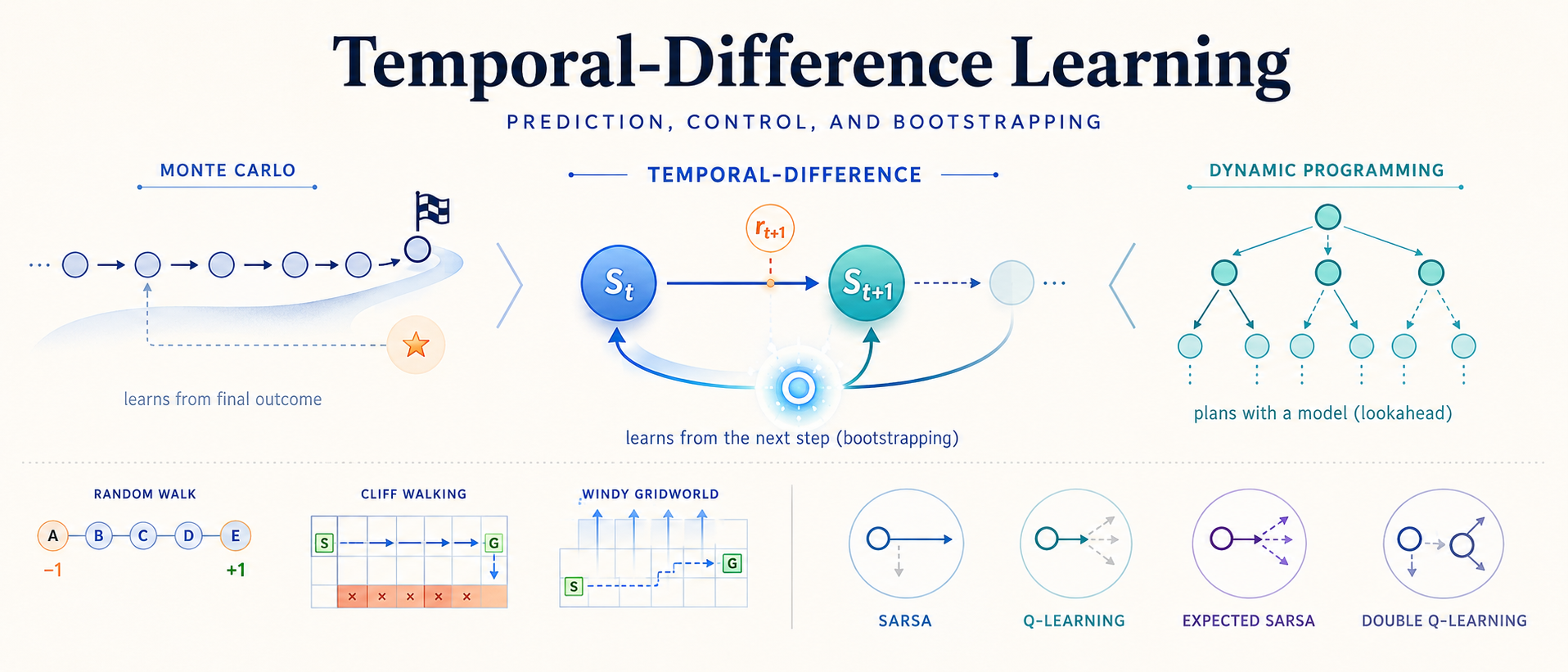
An illustration of TD Learning

This post captures my takeaways from Chapter 6 of the book Reinforcement Learning: An Introduction by Sutton and Barto, the bible of RL.

Background

TD learning is the combination of Monte Carlo and Dynamic Programming that were discussed in my previous blog posts. All the basic concepts of learning from raw experiences, not needing model of environment, and GPI framework are borrowed from MC methods. While, idea of using bootstrapping to estimate value functions is borrowed from DP. While this chapter acts as a beginning of unifying these three algorithms, further chapters build upon these ideas to develope powerful RL algorithms.

The One-Step Updates : TD Prediction

Like MC, TD also utilizes experiences to solve the prediction problem. Below is the Monte Carlo update rule for state-value function which MC utilizes for finding optimal policy. This is referred to as constant-$\alpha$ MC.

$V(S_t) \leftarrow V(S_t) + {\alpha} [G_t - V(S_t)]$

Where $G_t$ is the return from state $S_t$ to the end of the episode. While MC waits until the termination of episode to calculate $G_t$, TD on other hand updates the value function at each step $t$ as new reward is observed like shown below:

$V(S_t) \leftarrow V(S_t) + {\alpha} [R_{t+1} + \gamma V(S_{t+1}) - V(S_t)]$

Where $R_{t+1} + \gamma V(S_{t+1})$ is the target for the TD update. This is called TD(0) or One-step TD. This is boottsrapping method as we update estimates from estimates, i.e., we use $V(S_{t+1})$ to update $V(S_t)$. This way TD combines the sample update idea (looking ahead to a sample successor state) from Monte Carlo and Bootstrapping from DP.

DP uses expected updates which is based on distribution of all possible successors

def td0_prediction(env, policy, num_episodes, alpha):
    V = defaultdict(float)
    
    for _ in range(num_episodes):
        S, _ = env.reset()
        
        while not env.is_done(S):
            A = policy(S)
            next_S, R, done = env.step(A)
            
            # TD target and error
            td_target = R + env.gamma * V[next_S]
            td_error = td_target - V[S]
            
            # Update value function
            V[S] = V[S] + alpha * td_error
            
            S = next_S
    
    return V

The term $R_{t+1} + \gamma V(S_{t+1}) - V(S_t)$ is known as TD Error ($\delta_t$) which is difference between the one-step lookahead estimate of the return ($R_{t+1} + \gamma V(S_{t+1})$) and current value estimate ($V(S_t)$).

$\delta_t$ is error for $V(S_t)$ available at $t+1$.

In Monte carlo, the array V doesn't change during an episode, then the MC errors can be written as sum of TD errors.

This doesn't work if V is updated during episode (like TD(0)) but it still works if the updates are small and approximations are considered.

The Online Learner : Advantages of TD prediction Methods

One main direct advantage of TD over DP is that DP doesn't require model of environment and can directly compute the optimal policy by learning from experience. Unlike MC, TD can be implemented in online fashion not requiring to wait until end of an episode to update value function. This is very helpful for scenarios where there are longer episodes and situations where there is no concept of episode (continuous tasks). The idea of soft policy used in MC methods to tackle the scenario of visiting less probable states slows the learning whose effect is reduced in TD methods.

While there is no mathematical proof for which methods (MC or TD) converges faster, TD methods are usually found to converge faster than constant-$\alpha$ MC methods on stochastic tasks.

There is a good example in the book (Example 6.2) based on Random Walk proving this faster convergence for TD methods.

The Batch learner : Optimality of TD(0)

In the scenarios where there is a fixed experience (e.g. 50 episodes), one can repeatedly use it to update the value function. This is similar to incremental learning but instead of using new data we use the same data over and over again. All the available episodes/experiences are processed again and again with new value function until the value function converges. This is called batch updating. Below is the high level idea of batrch updating for TD and MC.

def batch_update(episodes, V, alpha, gamma, method="TD"):
    """
    episodes:
        [
          [(S0, R1, S1), (S1, R2, S2), ...],
          [(S0, R1, S1), ...],
          ...
        ]

    method:
        "MC" or "TD"
    """

    while not converged(V):

        
        V_old = V.copy() # freeze current values for this full batch sweep
        delta = {s: 0.0 for s in V.keys()} # accumulate all increments here

        for episode in episodes:
            if method == "MC":
                G = 0.0
                for (S, R, S_next) in reversed(episode):
                    G = R + gamma * G
                    target = G # MC target = actual return
                    delta[S] += alpha * (target - V_old[S])
            elif method == "TD":
                for (S, R, S_next) in episode:
                    # terminal state has value 0
                    next_value = 0.0 if is_terminal(S_next) else V_old[S_next]
                    # TD target = reward + value of next state
                    target = R + gamma * next_value
                    delta[S] += alpha * (target - V_old[S])

        # apply update only once after processing the full batch
        for s in V.keys():
            V[s] = V_old[s] + delta[s]

    return V

Both TD(0) and MC with batch updating converge to same values (different for TD and MC) irrespective of $\alpha$ (step-size parameter). Batch MC methods always find estimates that minimizes mean squared error on training set, whereas TD(0) always finds estimates that would be correct for the maximum likelihood model of Markov process.

Maximum likelihood estimate of parameter is parameter value whose probability of generating data is maximum. The estimated transition probabilities from i to j is fraction of observed transitions from i to j and expected reward is average of rewards observed on transitions from i to j.

Given this MLM model, we can estimate the value function accurately if the model were exactly correct. This is called certainity-equivalence estimate (same as assuming that estimate of underlying value function was known certainly rather than being approximated). TD(0) typically converges to this value which is why TD(0) is faster than MC methods.

In batch updating, Monte Carlo can be seen as fitting the observed returns in the dataset, while TD(0) generalizes through the Markov structure implied by the data.

MC asks: For every time I saw state s, what return actually followed it?

TD asks: For every time I saw state s, where did it go next, and what is that next state worth?

The On-Policy Controller : Sarsa

Now that we understand prediction method for TD, we can use it for the control problem. Similar to MC and DP methods we use Generalized Policy Iteration (GPI) framework to solve control problems. Like MC methods, we also have On-policy and Off-policy variants of TD methods.

We move from state-value functions for action-value functions for GPI. The equation can written as:

For terminal states, $Q(S_{t+1},A_{t+1})$ is set to 0. The name Sarsa came from the fact that all the terms ($S_t, A_t, R_{t+1}, S_{t+1}, A_{t+1}$ - State, Action, Reward, State, Action) are used to update the value function.

Coming back to GPI, We continuaslly estimate $q_\pi$ for the policy $\pi$ and also change $\pi$ towards greedy policy wrto $q_\pi$ until convergence. The convergence depends on type of policy used ($\epsilon$-greedy or $\epsilon$-soft). The pseudocode for Sarsa is as follows:

def sarsa(env, max_episodes, alpha, gamma, epsilon):
    """
    Sarsa algorithm for on-policy TD control.
    """
    # Initialize action-value function
    Q = np.zeros((env.nS, env.nA))

    # Epsilon-greedy policy
    def policy(state):
        if np.random.random() < epsilon:
            return np.random.randint(env.nA)
        else:
            return np.argmax(Q[state])

    # Main loop
    for episode in range(max_episodes):
        S = env.reset()
        A = policy(S)

        while True:
            S_next, R, done = env.step(A)

            # Break if episode ended
            if done:
                # Q[S, A] = Q[S, A] + alpha * (R - Q[S, A])
                break

            # Get next action from the same policy
            A_next = policy(S_next)

            # TD update rule for Sarsa
            Q[S, A] = Q[S, A] + alpha * (R + gamma * Q[S_next, A_next] - Q[S, A])

            # Update state and action
            S, A = S_next, A_next

    return Q

The Off-Policy Controller : Q-Learning

Incase of Off-policy TD we typically use policy $\pi$ ($\epsilon$-greedy behavior policy) for generating trajectories, but learn $q_*$ (greedy target policy) for the greedy policy wrto $q_*$. The equation for this update rule is as follows:

The learned action-value function $Q$ directly approximates the optimal action-value function $q_*$.

def q_learning(env, max_episodes, alpha, gamma, epsilon):
    """
    Q-Learning algorithm for off-policy TD control.
    """
    # Initialize action-value function
    Q = np.zeros((env.nS, env.nA))

    # Epsilon-greedy policy
    def policy(state):
        if np.random.random() < epsilon:
            return np.random.randint(env.nA)
        else:
            return np.argmax(Q[state])

    # Main loop
    for episode in range(max_episodes):
        S = env.reset()

        while True:
            A = policy(S)
            S_next, R, done = env.step(A)

            # Break if episode ended
            if done:
                Q[S, A] = Q[S, A] + alpha * (R - Q[S, A])
                break

            # Q-Learning update: always pick the best next action for the target
            best_next_action = np.argmax(Q[S_next])
            Q[S, A] = Q[S, A] + alpha * (R + gamma * Q[S_next, best_next_action] - Q[S, A])

            S = S_next

    return Q

The Averaging Controller : Expected Sarsa

Expected Sarsa is similar to Q-Learning but instead of maximum over next state action pairs, expected value is computed using the on-policy policy to consider how likely is each action under current policy.

$Q(S_t,A_t) \leftarrow Q(S_t,A_t) + \alpha \left[ R_{t+1} + \gamma \mathbb{E}_{\pi}[Q(S_{t+1},A_{t+1})|S_{t+1}] - Q(S_t,A_t) \right]$

Expected Sarsa removes the problem of variance in Sarsa by taking expected value instead of random action selection.

def expected_sarsa(env, max_episodes, alpha, gamma, epsilon):
    """
    Expected Sarsa algorithm for on-policy TD control.
    """
    # Initialize action-value function
    Q = np.zeros((env.nS, env.nA))

    # Epsilon-greedy policy
    def policy(state):
        if np.random.random() < epsilon:
            return np.random.randint(env.nA)
        else:
            return np.argmax(Q[state])

    # Main loop
    for episode in range(max_episodes):
        S = env.reset()

        while True:
            A = policy(S)
            S_next, R, done = env.step(A)

            # Break if episode ended
            if done:
                Q[S, A] = Q[S, A] + alpha * (R - Q[S, A])
                break

            # Expected Sarsa update: average over all possible next actions
            expected_next_value = 0.0
            for a_next in range(env.nA):
                prob = epsilon / env.nA  # probability of taking this action
                if a_next == np.argmax(Q[S_next]):
                    prob += 1 - epsilon  # if greedy, add extra probability
                expected_next_value += prob * Q[S_next, a_next]

            Q[S, A] = Q[S, A] + alpha * (R + gamma * expected_next_value - Q[S, A])

            S = S_next

    return Q

Backup diagrams for Sarsa, Q-Learning and Expected Sarsa are as follows:

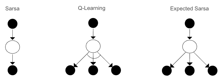Backup Diagrams

Cliff Walking Problem

Cliff Walking is a classic gridworld environment used to demonstrate the differences between various Temporal-Difference (TD) learning algorithms. Specifically, it elegantly highlights the behavioral distinctions between on-policy and off-policy control methods.

If you're not familiar with the Cliff Walking problem, it originates from Example 6.6 in Sutton and Barto's foundational book, Reinforcement Learning: An Introduction.

Mechanics

• Grid: The environment is a simple 12x4 rectangular grid.
• Objective: The agent begins in the bottom-left corner (Start) and must navigate to the bottom-right corner (Goal).
• Cliff: The entire bottom row of the grid, spanning directly between the start and goal states, is a dangerous "cliff". If the agent steps off the cliff, it incurs a penalty of -100 and is instantly sent back to the starting square.
• Movement: The agent can choose to move one square in any of the four cardinal directions: Up, Down, Left, or Right. Any movement that would take the agent off the grid leaves its state unchanged.

Framing the Game as an RL Problem

Cliff Walking is an episodic, finite Markov Decision Process (MDP) designed specifically to penalize risky behavior during the exploration phase.

• Rewards:
  • Each standard step taken yields a reward of -1. This incentivizes the agent to reach the goal taking as few steps as possible.
  • Stepping into the cliff region yields a severe penalty of -100.
• State Space: The grid consists of exactly 48 distinct states, represented by their (x, y) coordinate grid positions.
• Action Space: 4 discrete deterministic actions (Up, Down, Left, Right).

The TD Control Dilemma: Safe vs. Optimal

This environment brilliantly exposes the difference between On-Policy (Sarsa) and Off-Policy (Q-Learning) algorithms:

• Q-Learning learns the values of the absolutely optimal policy. It learns that taking the shortest path—walking right along the treacherous edge of the cliff—is the fastest way to win. However, because it explores randomly using an $\epsilon$-greedy policy during training, it frequently accidentally falls off the cliff, incurring terrible average returns.
• Sarsa takes the exploration strategy into account. It realizes that occasionally exploring near the cliff leads to falling, so it learns a safer, more conservative path higher up the grid.

Interactive Demo

Below is an interactive Temporal-Difference (TD) Learning Visualizer. It allows you to run and compare multiple TD algorithms side-by-side, letting you observe how different approaches naturally gravitate towards safe vs. risky paths in real-time.

Configurable Algorithms:

• Sarsa (On-Policy)
• Q-Learning (Off-Policy)
• Expected Sarsa

You can independently tweak the Learning Rate ($\alpha$) and Exploration Rate ($\epsilon$) for each run. You can also enable Double Learning to decouple action selection from evaluation (preventing maximization bias), or toggle Batch TD, which updates values repeatedly over mini-batches leading to much stabler convergence without high-frequency episodic noise.

• The Grid & Path Visualization: Watch the learned paths overlay directly onto the environment. Using the episode slider, you can observe how paths begin as chaotic random walks and slowly converge. (Look for Sarsa traversing the top of the grid, while Q-Learning hugs the cliff edge).
• State-Value Heatmap: Toggle the Heatmap V/Q switch to visualize how the agent perceives the board. (Notice how the cells immediately above the cliff are highly penalized by Sarsa (darker) but valued much higher by Q-Learning.)
• Learning Progress Chart: A comparative line graph of Cumulative Return vs. Episodes. This clearly illustrates the "cost of exploration". You can see Q-Learning suffer highly negative average returns during training due to cliff falls, while Sarsa quickly stabilizes to a higher average reward profile.

References

1. Sutton, R. S., & Barto, A. G. (2018). Reinforcement Learning: An Introduction.

Tools

• Image Generation: Gemini, ChatGPT
• Editor: Antigravity
• Flowchart and Diagrams: Excalidraw, Slides
• Interactive Demo: Google AI Studio