Dynamic Programming - Planning with a Perfect Model

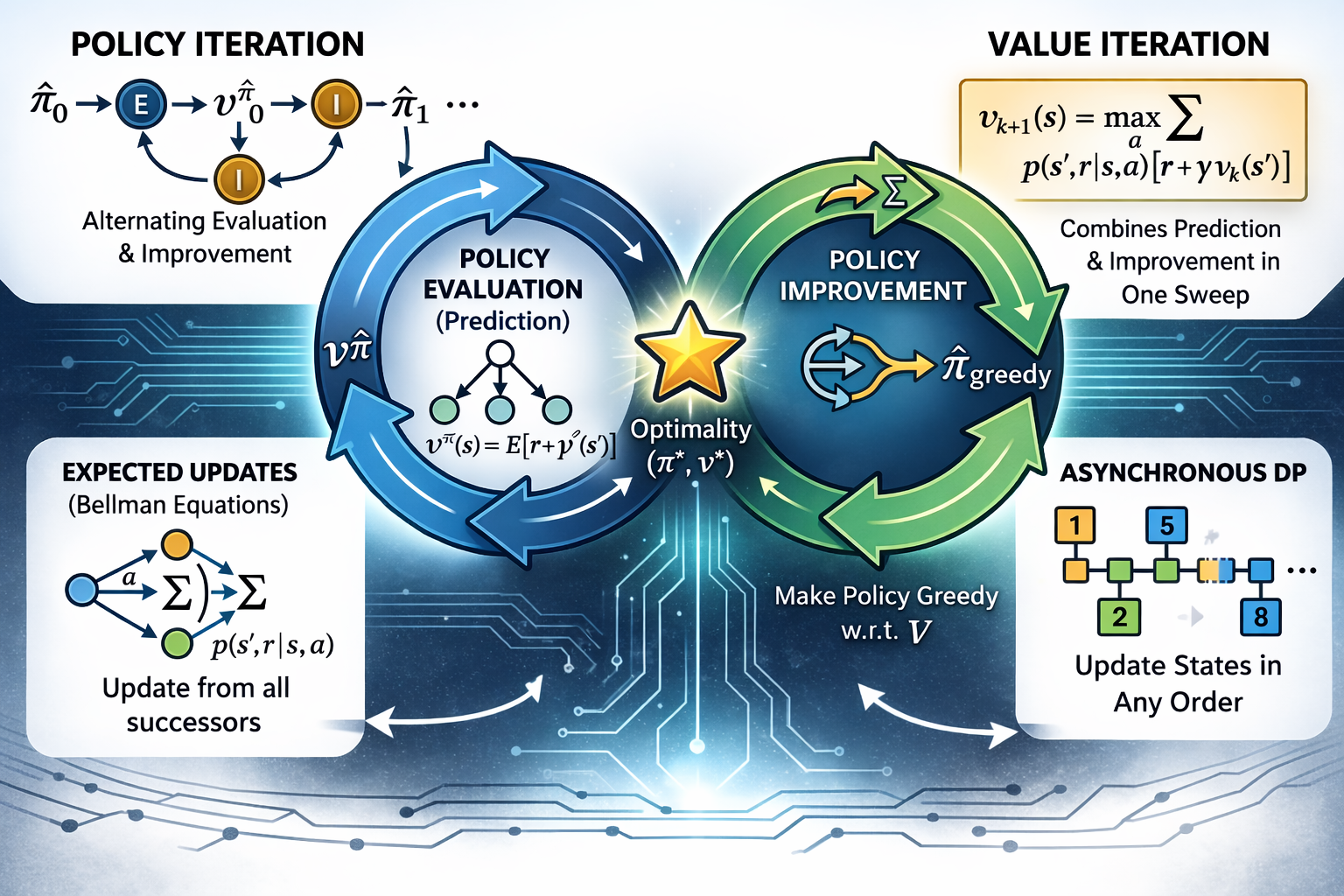
An illustration of Dynamic Programming

This post captures my takeaways from Chapter 4 of the book Reinforcement Learning: An Introduction by Sutton and Barto, the bible of RL.

Before starting this post, I would recommend you to go through Finite MDP post to better understand the concepts.

The Setup: A perfect model of the environment

Dynamic Programming (DP) is a class of algorithms used to compute optimal policies for MDPs when a perfect model of the environment is available. Even though their practical applicability is limited due to the requirement of a perfect model and computational cost, they provide a solid foundation for understanding the core concepts of RL. All the algorithms and concepts that will discussed further in the blogs/book are in some or the other way tries to achieve what a DP could achieve but with imperfect model and less computational cost.

What is a perfect model?

A perfect model of the environment is the complete knowledge of the environment dynamics. We assume that the environment is a Finite MDP further in this chapter. Revisiting Finite MDP, we know that the environment is defined by finite State, Action and Reward sets $(\mathcal{S}, \mathcal{A}, \mathcal{R})$ and dynamics are given by probabilities defined by $p(s', r | s, a)$.

DP can also be applied to continuous state and action spaces but it requires certain approximations and assumptions.

In this blog we will discuss about the key idea of DP (any RL algorithm in general) which is to use value functions as a tool to evaluate and improve policies. One way to think about this is to solving the Bellman Optimality Equations discussed in Finite MDP and using them as update rules to improve the policy.

The Assessment : Policy Evaluation

Computing the value function $v_\pi$ for a given policy $\pi$ is called as policy evaluation, also referred to as Prediction problem.

Considering the environment dymanics are knwown, above equation is a nothing but a system of linear equations in $S$. Consider a sequence of value functions $v_0, v_1, v_2, ...$ where $v_k(s)$ with initial $v_0$ chosen randomly. Each successive approximation of value function (using Bellman equation) is given by:

The algorithm is called Iterative Policy Evaluation. The sequence $\{v_k\}$ converges to $v_\pi$ as $k \to \infty$. For each successive approximation, the following update is applied to all states: old values of succcessor states of $s$ and expected immediate rewards along all the one-step transitions possible are used to update the old value of $s$. These updates are called expected updates as they are based on the expected values of the successor states and rewards. This process is repeated for all the states for all the policy evaluation steps to update the value function.

Coming to the implementation part, two approaches can be used:

• we maintain two arrays, one for the old value function and another for the new value function. We update the new value function using the old value function and then copy the new value function to old value function for next iteration. This process is repeated until the value function converges to $v_\pi$.
• we can also update the value function in place, i.e., we can update the value function for each state using the old values of successor states and rewards. This process is repeated until the value function converges to $v_\pi$. Notable inplace-update converges faster than the first approach. The psuedocode for the inplace-update approach is given below:

def policy_evaluation(env, policy, theta=1e-6):
    V = np.zeros(env.nS)  # Initialize value function
    while True:
        delta = 0
        for s in range(env.nS):
            v = V[s]  # Store old value
            new_v = 0
            for a in range(env.nA):
                action_prob = policy[s][a]
                for prob, next_state, reward, done in env.P[s][a]:
                    new_v += action_prob * prob * (reward + V[next_state])
            V[s] = new_v  # Update value function
            delta = max(delta, abs(v - new_v))  # Update delta
        if delta < theta:  # Check for convergence
            break
    return V

The Upgrade : Policy Improvement

Now that we know how to update value function, we can focus on using it find a better policy. Before that, let's recall the Bellman Optimality Equation for action-value function:

One way to know would be select an action $a$ in states $s$ and check if it's greater than $v_\pi(s)$, if it is, then we can conclude that it's better to take $a$ and follow $\pi$ thereafter rather than following $\pi$ from the start. This is the key idea behind policy improvement. Building on top of that we can even argue that the policy where taking action $a$ everytime $s$ encountered is better than or equal to $\pi$. This is the policy improvement theorem which states that if for all states $s$, $q_\pi(s, \pi'(s)) \geq v_\pi(s)$, then the policy $\pi'$ is better than or equal to $\pi$.

A policy $\pi'$ is better than or equal to a policy $\pi$ if $q_\pi(s, \pi'(s)) \geq v_\pi(s)$ for all states $s$. This relation also holds for $v_\pi'(s) \geq v_\pi(s)$

I recommend to deduce this later relation using the former equation on your own.

This change in policy at a single state can further be extended to all states, selecting the action that maximizes $q_\pi(s, a)$ for each state $s$. This greedy policy $\pi'$ is given by:

This greedy policy selects an action that maximizes the return in short-term by one step lookahead according to $v_\pi$. This process finding a new policy by acting greedily with respect to the value function of original policy is called Policy Improvement. If you look at it, the greedy policy follows the policy improvement theorem. Policy improvement strictly gives a better policy unless until the original policy is already optimal.

We have only discussed about deterministic policies but the idea can be extended to stochastic policy cases where $\pi(a|s)$ gives the probability of taking action $a$ in state $s$.

The Cycle : Policy Iteration

Now that we have the tools to evaluate and improve policies, we can combine them to find the optimal policy. The process of alternating between policy evaluation and policy improvement is called Policy Iteration. The algorithm starts with an arbitrary policy and then iteratively evaluates the value function for the current policy and improves the policy using the greedy approach until convergence.

This sequence converges to optimal policy and value functions considering we are in a finite MDP. This process is called Policy Iteration. The pseudocode for policy iteration is given below:

def policy_iteration(env, theta=1e-6):
    # Initialization
    policy = np.ones([env.nS, env.nA]) / env.nA
    while  True:
        # Policy Evaluation
        for s in range(env.nS):
            V[s] = 0
            for a in range(env.nA):
                action_prob = policy[s][a]
                for prob, next_state, reward, done in env.P[s][a]:
                    V[s] += action_prob * prob * (reward + V[next_state])
                    theta = max(theta, abs(V[s] - v_old[s]))  
        if theta < 1e-6:  # Check for convergence
            break

        # Policy Improvement
        policy_stable = True
        for s in range(env.nS):
            old_action = np.argmax(policy[s])  # Store old action
            policy[s] = np.zeros(env.nA)
            policy[s][np.argmax(V[s])] = 1  # Greedy policy
            if old_action != np.argmax(policy[s]):
                policy_stable = False
        if policy_stable:
            return policy, V

The Shortcut : Value Iteration

Policy Iteration is a powerful algorithm but it can be computationally expensive as it requires multiple iterations of policy evaluation. Each policy evaluation step inturn requires multiple sweeps through state set. The exact convergence of policy evaluation only happens in the limit of infinite iterations. Even though we stop using a threshold $\theta$, it still undergoes many sweeps through the state set. Inshort, waiting for perfect convergence during evaluation phase slows down the actual goal of finding the optimal policy.

One efficient way of truncating this policy evaluation step is by stopping after just one sweep through the state set. This algorithm is called Value iteration. This algorithm combines policy improvement and truncated policy evaluation into a single step. The update rule for value iteration is given by:

Similarly we can also write the action-value version of the update rule as:

The value iteration equation is similar to policy evaluation equation: instead of taking the expectation over actions according to the policy, we take the maximum over actions. The backup diagrams shown below of both policy evaluation and value iteration can help better understand the difference between the two algorithms.

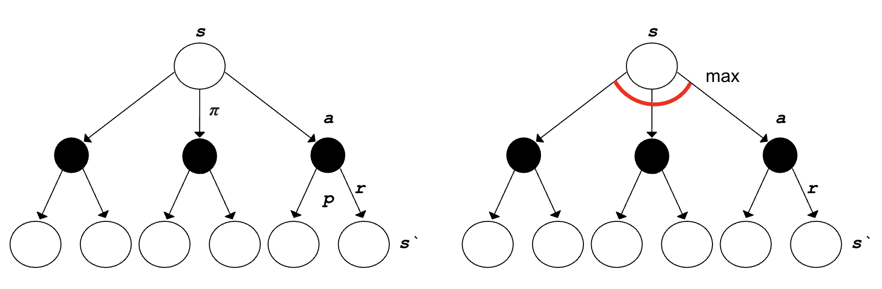Policy Evaluation (Left) vs Value Iteration (Right)

The pseudocode for value iteration is given below:

def value_iteration(env, theta=1e-6):
    V = np.zeros(env.nS)  # Initialize value function
    while True:
        delta = 0
        for s in range(env.nS):
            v = V[s]  # Store old value
            new_v = float('-inf')
            for a in range(env.nA):
                action_value = 0
                for prob, next_state, reward, done in env.P[s][a]:
                    action_value += prob * (reward + V[next_state])
                new_v = max(new_v, action_value)  # Update new value
            V[s] = new_v  # Update value function
            delta = max(delta, abs(v - new_v))  # Update delta
        if delta < theta:  # Check for convergence
            break
    # Derive policy from value function
    policy = np.zeros([env.nS, env.nA])
    for s in range(env.nS):
        best_action = np.argmax([sum(prob * (reward + V[next_state]) for prob, next_state, reward, done in env.P[s][a]) for a in range(env.nA)])
        policy[s][best_action] = 1  # Greedy policy
    return policy, V

In general the truncated policy iteration algorithms are sequences of policy evaluation updates with some using value iteration updates.

Gambler's Problem

The Gambler's Problem is a classic example in DP. It involves a gambler who bets on the outcome of a coin flip, with the goal of reaching a certain amount of money (the goal state) before going broke (the terminal state). If the coin flips turns out to be a heads, he wins as much stake as he bets and loses his stake if it's tails. On each coin flip, gambler needs to decide what part of his current capital to bet. This problem nothing but a episodic, finite MDP.

Problem Setup

The state ($s$) is the gambler's capital which can range from $0$ to $99$ and actions are stakes $a \in {0, 1, \ldots, min(s, 100-s)}$. The game ends when gambler reaches either $0$ (terminal) or $100$ (goal). The reward is $+1$ if the gambler reaches the goal state and $0$ otherwise. Policy is mapping from capital to the stake. Probability $p_h$ denotes the probability of coin landing heads. Entire problem can be solved with a given $p_h$ using value iteration. Let us solve the problem for 3 different values of $p_h$ (0.25, 0.5 and 0.75) and see how the optimal policy and value function changes with it.

Value Iteration Implementation

goal = 100
ph = 0.4
theta = 1e-9
V = np.zeros(goal + 1)
V[goal] = 1
S = np.arange(1, goal)

v_track = [V.copy()]

# Value Iteration
while True:
    delta = 0

    for s in S:
        v = V[s]

        act_returns = []
        actions = np.arange(1, min(s, goal - s) + 1)
        for a in actions:
            exp_return = ph * V[s+a] + (1 - ph) * V[s-a]
            act_returns.append(exp_return)

        V[s] = max(act_returns)
        delta = max(delta, abs(v - V[s]))

    v_track.append(V.copy())

    if delta < theta:
        break

# Optimal policy
policy = np.zeros(goal + 1)
for s in S:
    act_returns = []
    actions = np.arange(1, min(s, goal - s) + 1)
    for a in actions:
        exp_return = ph * V[s+a] + (1 - ph) * V[s-a]
        # Round to 5 decimal places to avoid floating point issues
        act_returns.append(np.round(exp_return, 5)) 

    best_action = np.argmax(act_returns)
    policy[s] = best_action

Below are the optimal value functions and policies for different values of $p_h$:

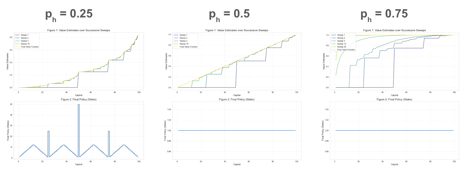Optimal Value Functions for different $p_h$ values (0.25, 0.5, 0.75). Top plot shows value function at different sweeps. Bottom plot shows optimal policy.

Notice how the value function shape changes from convex to flat to concave with increasing $p_h$. Also the optimal policy flattens starting from $p_h=0.5$. There are 3 different scenarios for the gambler's problem:

• $p_h < 0.5$: The gambler is more likely to lose than win. The optimal policy becomes highly aggressive. To minimize exposure to the disadvantage of losing, the agent makes massive bets to try and hit the goal as quickly as possible.
• $p_h = 0.5$: The expected return of any bet is exactly zero, making the value curve a perfectly straight diagonal line. Because every possible betting strategy yields the exact same overall win probability, the flat policy of betting 1 is simply a tie-breaker because how the code is written (np.argmax()).
• $p_h > 0.5$: The gambler is more likely to win than lose, so decides to have maximum exposure (unlike $p_h<0.5$). By betting the absolute minimum (1) stake every time, the agent eliminates the risk of ruin and lets its higher probability advantage safely guarantee the win. That's why we generally see this case goes on for a long time before hitting the goal.

The Bottleneck : Computational Cost

Even though we have reduced the computational cost by moving from policy iteration to value iteration, we still need to sweep through entire state set for each iteration. For games like Chess, Go, Backgammon etc, the state space is huge and it becomes computationally infeasible to sweep through the entire state space for each iteration.

Asynchronous dynamic programming algorithms are a class of algorithms that update the value function for only a subset of states at each iteration. These algorithms updates the values of states in any order, using whatever values of states available. This gives flexibility to control what states to update at each iteration. Asynchronous DP makes it easier to do intermix computation with real-time interaction (similar to online learning in Deep learning). States can updated as the agent visits them in real-time. The agent's experience can be used to determine what states to update at each iteration.

Universal Framework : Generalized Policy Iteration (GPI)

Policy Iteration consists of two components interacting with each other:

• Value function being consistent with the policy (policy evaluation)
• Policy being greedy with respect to the value function (policy improvement)

These two processes alternate and compete with eachother (if you're familiar with GANs, you can understand it better with that analogy). The term Generalized Policy Iteration (GPI) is used to refer to the idea of having two processes, policy evaluation and policy improvement, that interact with each other, independent of details of two processes. Any RL method can be described as GPI:

• Policy function always being improved with respect to the value function
• Value function being driven towards value function for the current policy

The value function stabilizes only when it is consistent with current policy and the policy stabilizes only when it is greedy with respect to the current value function. These two process are both cooperating and competing with eachother. Making policy function greedy wrto value function makes value function incorrect for the new policy and making value function consistent with the new policy makes the policy non-greedy wrto the new value function. This process continues until both of them stabilize to optimal policy and optimal value function.

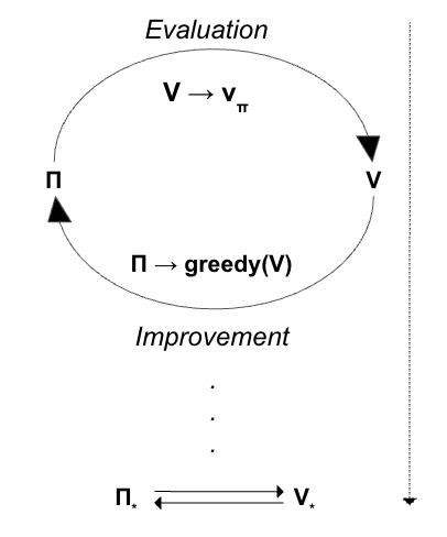A diagram showing the interaction between policy evaluation and policy improvement processes.

Interactive Demo

To better understand the concepts of DP, I have created an interactive demo of DP algorithm's working on a small gridworld environment.

• State ($s$): A specific cell on the 4x4 grid.
• Action ($a$): The move the agent takes (Up, Down, Left, Right).
• Reward ($R$): Feedback received after a move.
  • -1: Standard move cost (living penalty).
  • -10: Trap penalty.
  • 0: Goal reward (Terminal state).
• Value Function ($V(s)$): The expected total future reward from a state. Higher values (green) are better; lower values (red) are worse.
• Policy ($\pi$): The strategy (arrows) indicating the best action to take from a state.

The app runs three algorithms simultaneously to find the Optimal Policy:

1. Policy Iteration
2. Value Iteration
3. Truncated Policy Iteration: A hybrid approach. Runs Policy Evaluation for a fixed number of steps ($k=5$) instead of waiting for full convergence before improving the policy.

Instructions

• Hover: See the exact Bellman Equation calculation for that cell in the Math Inspector.
• Click: Edit the cell type based on the selected Editor Mode.
• Visuals:
  • Arrows: Best direction to move.
  • Heatmap: Green = High Value, Red = Low Value.
• Play/Step: Run the simulation.
• Speed: Adjust iteration speed.
• Gamma ($\gamma$): Discount factor (0-1). Higher $\gamma$ means the agent cares more about long-term rewards.
• Async Mode:
  • Off: Synchronous updates (all cells update at once).
  • On: Asynchronous updates (cells update one-by-one using latest values).
• Editor Modes: Place Walls (obstacles) or Traps (hazards).
• Convergence Plot: Tracks the maximum change in values ($\Delta$) over time. When the line hits 0, the algorithm has converged.

References

1. Sutton, R. S., & Barto, A. G. (2018). Reinforcement Learning: An Introduction.

Tools

• Image Generation: Gemini, ChatGPT
• Editor: Antigravity
• Flowchart and Diagrams: Excalidraw, Slides
• Interactive Demo: Google AI Studio