
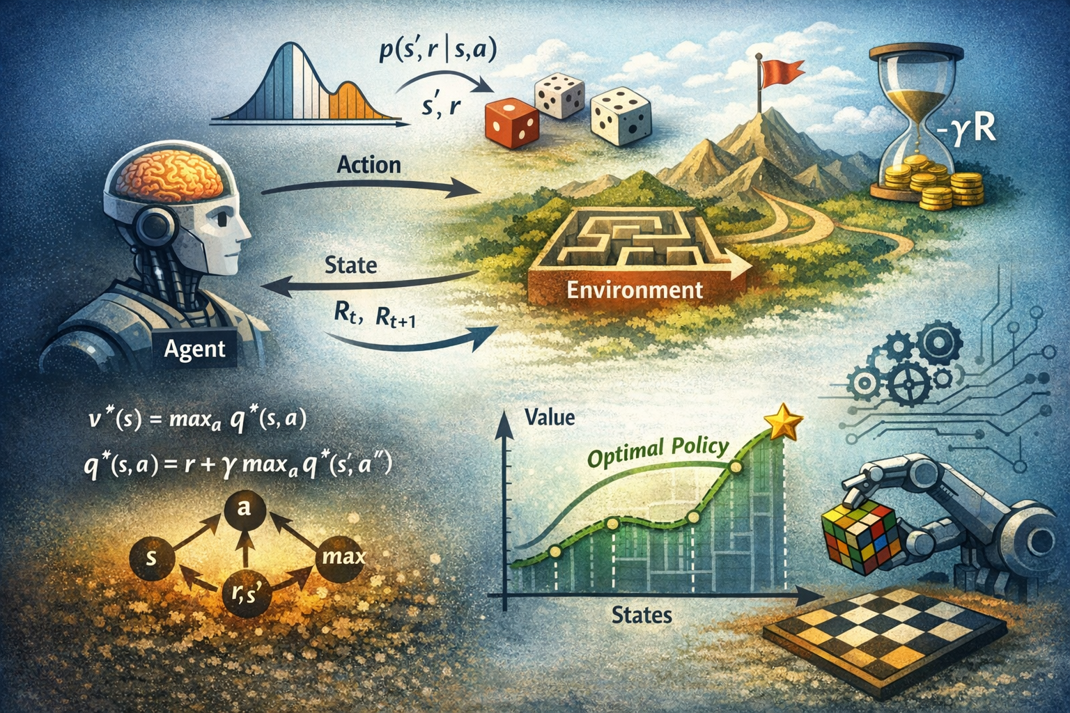
 An illustration of Finite MDP
This post captures my takeaways from Chapter 3 of the book Reinforcement Learning: An Introduction by Sutton and Barto, the bible of RL.
The Setup : Agent and Environment
Recap from Intro to RL and Multi-Armed Bandits, we have seen that agent, a learner and decision maker interacts with an environment. At each step, the agent observes the state of the environment and takes an action. The environment then transitions to a new state and provides a reward to the agent. Agent seeks to maximize the rewards it receives over time by selecting optimal actions. Markov Decision Process (MDP) is a mathematical framework for modeling such interactions in RL.
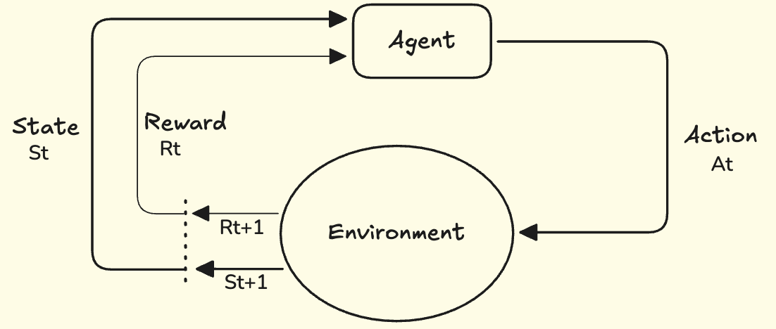 Interaction between Agent and Environment in a MDP
The continuous interactions described in above figure results in sequence of observations, actions and rewards:
In a finite MDP, the state, action and rewards have finite number of elements. Let's denote the set of states by , actions by , and rewards by . The random variables are probability distributions dependent on previous state and action.
When is it a MDP?
The function completely defines the dynamics of MDP. In MDP, the and only depends on and and not on any previous states and actions. The state must contain all the past agent-environment interactions information. The state that follows this is said to have the Markov Property. Using the above equation we can formalize any information that we would like to know about the environment:
State Transition Probabilities
Expected Rewards
State-Action pairs
State-Action-Next State tuples
I encourage you to deduce the above equations and generate more such formulations you can think of. For example, what is the expected reward for a state-action-next_state-reward tuple? Go through Chain rule and bayes theorem to understand the above equations in-depth.
Applications
MDP framework is flexible and can be applied to a wide range of problems. Time-steps need not be a fixed intervals of time, it can refer to any successive stages of interaction between agent and environment. The actions can be as simple as the voltage control in robot arm to as complex as the stock trading decisions. The states can be as simple as the position of the robot arm to as complex as the current market conditions. In general actions can be any decisions we want to learn how to make and state can be anything that helps us make those decisions.
The boundary between agent and environment is also not rigid. For example, in a robot arm problem, the motor control system can be considered part of the environment or part of the agent. In general anything that is not in our control is environment. The agent-environment boundary only signifies the limit og agent's control, not of it's knowledge. Reward computation is considered to be external to the agent, because it defines the task to the agent and agent should not have control over it.
MDP framework is a very powerful yet simple abstraction of goal directed learning which reduces the problem into three signals passing back and forth between agent and environment: State, Action and Reward.
The Payoff : Goals and Rewards
The agent's goal is to maximize cumulative reward in long run, which is called as reward hypothesis. This idea of formalizing goal by using rewards is a very distincitive feature of reinforcement learning. The definition of reward signal should be indicative of what we want the agent to achieve and any prior knowledge about how to achieve the goal should not be imparted on agent.
The reward signal is a way of communicating what we want to achieve and not how to achieve it.
The Timeline : Returns and Episodes
A simple way to define the cumulative reward is to sum up all the rewards the agent receives over time. This approach makes sense for tasks that have a clear start and end which are called as episodes and the tasks as episodic tasks. Each episode ends in a special state called as terminal state. Every episode begins independently of the previous episodes and the agent starts from the same initial state. The time of termination T varies from episode to episode.
The tasks which do not have a naturally identifiable episodes are called as continuing tasks. The above formula if used here will result in infinite sum. To avoid this we introduce a discount factor which is a factor by which we discount the future rewards. This concept is called as discounting. A reward recieved k time steps in future is worth only times if it's recieved immediately. The special case of makes the agent myopic, only caring about immediate rewards. The special case of makes the agent far-sighted, caring about all the future rewards equally.
The Bridge : Unified Notation for Episodic and Continuous tasks
In episodic tasks, every episode starts with a time step of zero. So, it becomes essential to track the episode number along with the time step ( as ). But when we disucss about episodic tasks, we always talk or think about a single episode, which makes the notation redundant.
One more thing to note is about infinite time steps in continuous tasks. To unify both episodic and continuous tasks, we introduce a special episode called absorbing state for episodic tasks. This state transitions to itself and has zero reward.
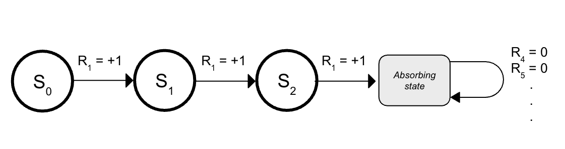 Episodic Task with absorbing state
The generalized return for both episodic and continuous tasks is given by (handles or cases but not both):
The Strategy : Policy and Value functions
- Value Function: Estimates how good it is to be in a state or take an action in a state. "How good" is measured by the expected return that is discussed in the previous section.
- Policy: A policy is a function that assigns to each state the probability of choosing each available action. It determines how the agent behaves at a particular moment, and value functions are defined in relation to these specific policies. Let agent follows a policy at time , then the probability of choosing action in state is given by - Probability that given .
State-Value Function
The value function of a state under a policy denotes as is the expected return starting from state and following policy thereafter. This is also called as state-value function for policy .
Action-Value Function
The value of taking an action in a state under a policy denotes as is defined as action-value function for policy .
Bellman Equation
The value functions and are computed from experience i.e, if an agent follows a certain policy and keeps track of the returns folllowed by every state encountered, the state's value for every state as we iterate infinite times. Similarly, if separate averages are tracked for each state-action pair, they will converge to for every state-action pair. This method is called as Monte Carlo method (Next chapter).
This method is intangible when there are many states and actions where keeping track of all the averages is almost impossible. In such cases, we parametrize the and functions and adjust parameters to match the actual returns (not discussed in this post).
Value functions follows recursive relationships. For any policy , the value of a state can be written in terms of value of its successor states.
The last equation is called as Bellman equation. It is sum over all possible actions the agent can take, and for each action, it is sum over all possible next states and rewards the agent can receive. For each triple, we compute the probability term and multiply it with the reward term . This is represented as a backup diagram below. The backup operations transfers the value of successor states to the current state. These backup diagrams are used in many RL algorithms to provide visual intuition about the algorithm.
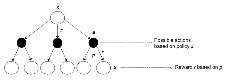 Backup diagram for
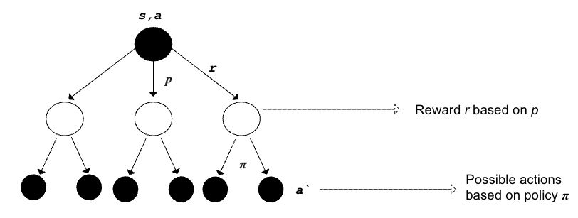 Backup diagram for
Below backup diagrams shows the dependencies between state-value and action-value functions.
- Top: The value of a state dependes on the values of actions possible from that state and how likely each action can be taken under current policy.
- Bottom: The value of an action depends on the expected next rewards and sum of remaining rewards.
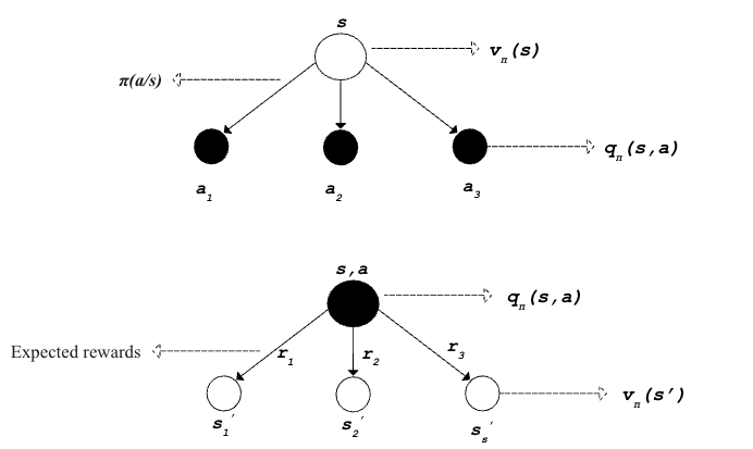 Backup diagrams for sta-value and action-value dependencies
The Solution : Optimal Policy and Value functions
A policy is said to be better than policy if it's expected return is greater than or equal for all states ( iff for all ). The policy which is better than all other policies is called as optimal policy and is denoted by . This optimal policy results in optimal state-value function and optimal action-value function and their Bellman optimal equations are:
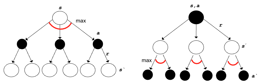 Backup diagram for and
For a finite MDP, the Bellman optimality equation for has unique solution. It is a system of equations, one for each state. If the the dynamics of environment () are known, then the optimal value function is obtained by solving system of non-linear equations.
Using we can find the optimal policy by choosing the action that maximizes the expected return for each state. A one-step search is performed to find the optimal policy. If we have then the optimal policy calculation doesn't require one step search as we cache the values of for each state-action pair. Hence, using , the optimal policy can be obtained without knowing about possible next states and rewards (but at the expense of representing as a function of state-action pairs).
Limitations
The above proposed method can only be used when:
- The dynamics of the enviuronment are accurately known
- Computational resources are available to solve the system of equations
- The states have the Markov property
Any real-case scenario violates at least one of the above conditions. For instance, in a chess game, the number of states is too large to be performing a exhaustive search looking ahead all the possible moves and their feasibilities alongwith rewards. So, we generally settle at approximate solutions of Bellman optimality equations (actual solutions are out of scope of this blog).
Example : Warehouse Navigation Robot
Setup
The agent (robot) is placed in a warehouse represented as a grid with a goal to reach the target location. At each step, the agent can move in four directions (up, down, left, right) and the goal is to reach the shipping bay to deliver the package with minimum number of steps.
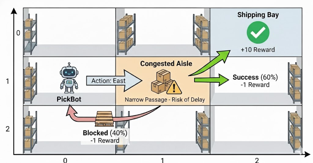 Warehouse environment
- States (): Coordinates where .
- Actions (): .
- Rewards ():
- -1 for every standard movement.
- +10 for reaching the Shipping Bay at (Terminal State).
- Congestion Penalty: Moving into or through state is risky.
- Dynamics ():
- In congested aisle ,
- Success (60%): The aisle is clear. It reaches with .
- Failuere (40%): A pallet blocks the path. The robot stays at and receives .
- In other aisles, the agent has 100% chance of moving in the desired direction.
- Agent can move in any direction with equal probability (1/4).
- In congested aisle ,
Return
A discount rate of is used to discount future rewards. Consider a trajectory where the robot attempts to enter the congested aisle, gets blocked once, succeeds on the second try, and then reaches the goal.
The Trajectory: (reaches goal at ).
The Calculation:
Bellman Equation
We want to find the value of the state under a policy where the robot always chooses to go East. Assume the neighboring state values are already known: and .
Applying the Equation:
Optimal Policy
The optimal policy is found by comparing the values of all possible actions. At state , the agent compares the value of the "Congested Shortcut" vs. the "Clear Long Way."
If the value of going North (avoiding the crowd) is and the value of pushing through the East aisle is , the Optimal Policy will deterministically choose North, even though it increases the physical distance to the goal.
References
- Sutton, R. S., & Barto, A. G. (2018). Reinforcement Learning: An Introduction.
Tools
- Image Generation: Gemini, ChatGPT
- Editor: Antigravity
- Flowchart and Diagrams: Excalidraw, Slides
Citation
Shanmukha Sainath. "Finite Markov Decision Processes - Sequential Decision Making". TensorWrites (Feb 2026). https://www.tensorwrites.com/posts/finite-mdp
@article{finitemdp2026,
  title   = "Finite Markov Decision Processes - Sequential Decision Making",
  author  = "Shanmukha Sainath",
  journal = "TensorWrites",
  year    = "2026",
  month   = "Feb",
  url     = "https://www.tensorwrites.com/posts/finite-mdp"
}