Multi-armed Bandits : Introducing evaluative aspect to RL

Header Overview of Multi-Armed Bandits and different RL Approaches

This post captures my takeaways from Chapter 3 of the book Reinforcement Learning: An Introduction by Sutton and Barto, the bible of RL.

The K-Armed Bandit Problem

An agent is told to repeatedly chose one of K available actions. Each action leads to a numerical reward that is sampled from a probability distribution corresponding to the action. The goal is to maximize the total reward over a fixed number of trials or time steps.

The name "K-armed bandit" comes from the idea of a slot machine but with K levers, each corresponding to an action. The reward distribution for each action is unknown to the agent, and the agent must learn the best action to take in order to maximize its total reward. Each of K actions has an expected or mean reward given that action is selected which we defines as value of that action denoted as $q_*(a)$ . Let $R_t$ be the reward at time $t$ and $A_t$ be the action taken at time $t$ . Then the expected reward for action $a$ is given by

q_*(a) = E[R_t | a]

If we maintain the estimate of action values, it can help the agent to make better decisions in the future. If we chose the action with the highest estimated value, we call it greedy action and we are exploiting our knowledge. But if we chose a random action, we call it random action and we are exploring the environment. Exploitation might yield immediate higher rewards but exploration may produce greater rewards in the long run. The decision to explore or exploit is a very complex trade-off that depends on accurate values of actions, uncertainities and the number of trials. This blog covers few simpler balancing methods to tackle exploration-exploitation dilemma.

Below is an example for a 10-armed bandit testbed. The "True Value" $q_*(a)$ of each arm is drawn from a $N(0, 1)$ distribution. Actual rewards are then drawn from $N(q_*(a), 1)$ .

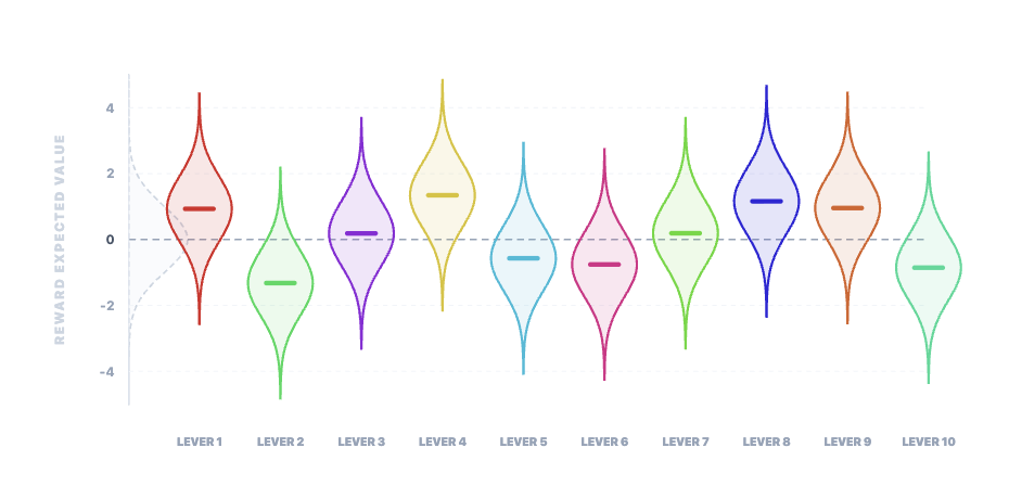Bandit Testbed The true value of each arm is drawn from a $N(0, 1)$ distribution (dotted line). Actual rewards are then drawn from $N(q_*(a), 1)$ (distributions for each arm)

We use this testbed to compare the performance of different action-value methods further in this blog.

Action-Value Methods

The methods ued for estimating values of actions and thereby using them to make decisions are called action-value methods. We start with a simpler and straight forward method called sample average method and build upon it to cover more complex methods for making action selection decisions.

Sample-Average Method

The sample average method is a simple and intuitive way to estimate the value of an action. It works by maintaining a running average of the rewards received for each action and using this average to make decisions. Let $Q_n(a)$ be the running average of the rewards received for action $a$ after $n$ trials. Then the running average is given by

Q_n(a) = \frac{1}{n} \sum_{i=1}^{n} R_i

$Q_n(a)$ converges to $q_*(a)$ as $n \to \infty$ by the law of large numbers.

Action selection

Greedy Action: The simplest way to select an action is to always choose the action with the highest estimated value. This is called greedy action. Let $A_t$ be the action taken at time $t$ . Then the greedy action is given by

A_t = \arg\max_{a} Q_n(a)

$\epsilon$ -greedy Action: Greedy action exploits the existing knowledge to maximize the immediate rewards. But it might miss out on a "jackpot" it didn't know existed. $\epsilon$ -greedy action explores the environment to gather new information. Let $A_t$ be the action taken at time $t$ . Then the $\epsilon$ -greedy action is given by

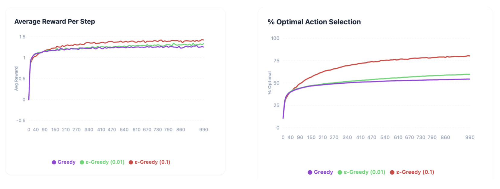A_t = \begin{cases} \arg\max_{a} Q_n(a) & \text{with probability } 1 - \epsilon \\ a & \text{with probability } \epsilon \end{cases}

Greedy vs ϵ-Greedy Left: Average reward per step estimated from 10000 episodes. Right: % Optimal Action selected. It is very evident that ϵ-greedy outperforms greedy and greater the value of ϵ, greater is the performance.

The Efficiency Hack: Incremental Implementation

Though the sample average method is simple and intuitive, as we increase the number of trials and episodes, computing the action-values efficiently is very important. Let $Q_n(a)$ be the running average of the rewards received for action $a$ after $n$ trials. Then the running average can be computed efficiently using the following update rule (it's very straight forward to derive, I recommend you to derive it on your own):

Q_n = \frac{1}{n} (R_1 + R_2 + ... + R_{n-1} + R_n) \\ Q_{n+1} = Q_n + \frac{1}{n} [R_{n} - Q_n]

This implementation reqquires use to keep store only $Q_n$ and $n$ to compute the next action value. This is very efficient in terms of space and computational complexity. The equation resembles the update rule that can be seen very frequently in Reinforcement Learning (even in Deep Learning).

NewEstimate = OldEstimate + StepSize \times [Target - OldEstimate]

The final pseudocode for simple bandit algorithm with $\epsilon$ -greedy action selection is given below:

\begin{aligned} \text{Initialize: } & Q(a) \leftarrow 0 \text{ for all } a \in \mathcal{A} \\ & N(a) \leftarrow 0 \text{ for all } a \in \mathcal{A} \\ \text{Repeat: } & \\ & A \leftarrow \begin{cases} \arg\max_{a} Q(a) & \text{with probability } 1 - \epsilon \\ \text{random action} & \text{with probability } \epsilon \end{cases} \\ & R \leftarrow \text{sample reward for action } A \\ & N(A) \leftarrow N(A) + 1 \\ & Q(A) \leftarrow Q(A) + \frac{1}{N(A)} [R - Q(A)] \end{aligned}

Adapting to Change: Non-Stationary Problems

The algorithm discussed above holds only for stationary problems where the reward distributions are constant over time. But in real world problems, the reward distributions may change over time. In such cases, we need to adapt our algorithm to handle non-stationary problems. In such cases it makes more sense to give more weight to recent rewards and less weight to older rewards. This can be achieved by using a learning rate that is constant over time. The update rule can be modified as follows:

Q_{n+1} = Q_n + \alpha [R_n - Q_n]

This is also called as exponential recency-weighte average as weight decays exponentially wrto exponent of $1-\alpha$ (Expand the above equation to $i^{th}$ reward $R_i$ to see it for yourself).

If we want to vary learning rate but in a different procedure from sample average method, we need to make sure that the learning rate satisfies certain conditions required for convergence. Let $\alpha_n(a)$ be the learning rate for action $a$ after its $n^{th}$ selection (equals $\frac{1}{n}$ for sample average method). Not all learning rates would lead to convergence. Based on stochastic pproximation theory 1, following conditions are required for the learning rate to lead to convergence:

\begin{aligned} & \alpha_n(a) \to 0 & \text{as } n \to \infty \\ & \sum_{n=1}^{\infty} \alpha_n(a) = \infty \end{aligned}

Solving the Dilemma: Encouraging Exploration

All the methods discussed abobe are biased by the initial actio-value estimates $Q_1(a)$ (which is set to 0 here). While the effect goes away in simple average method once all the actions are selected atleast once, it stays for the learning rate based methods. Though they become a set of user-defined parameters which is cumbersome, it allows use to provide some provide knowledge about the level of rewards and also helps to encourage exploration.

For example, in the 10-armed bandit problem, if we know that the best action has a reward of 5, we can set $Q_1(a) = 5$ for all actions. In the begining, even though the greedy action selection always selects the best action, the reward obtained is very less then initial estimate of 5. So the agent switches to other actions to explore the environment. This technique is known as optimistic initial values. This method doesn't work for non-stationary problems (the exploration power is temporary which doesn't work in a variable environment) but it is a good starting point to introduce exploration in the agent jusst like $\epsilon$ -greedy.

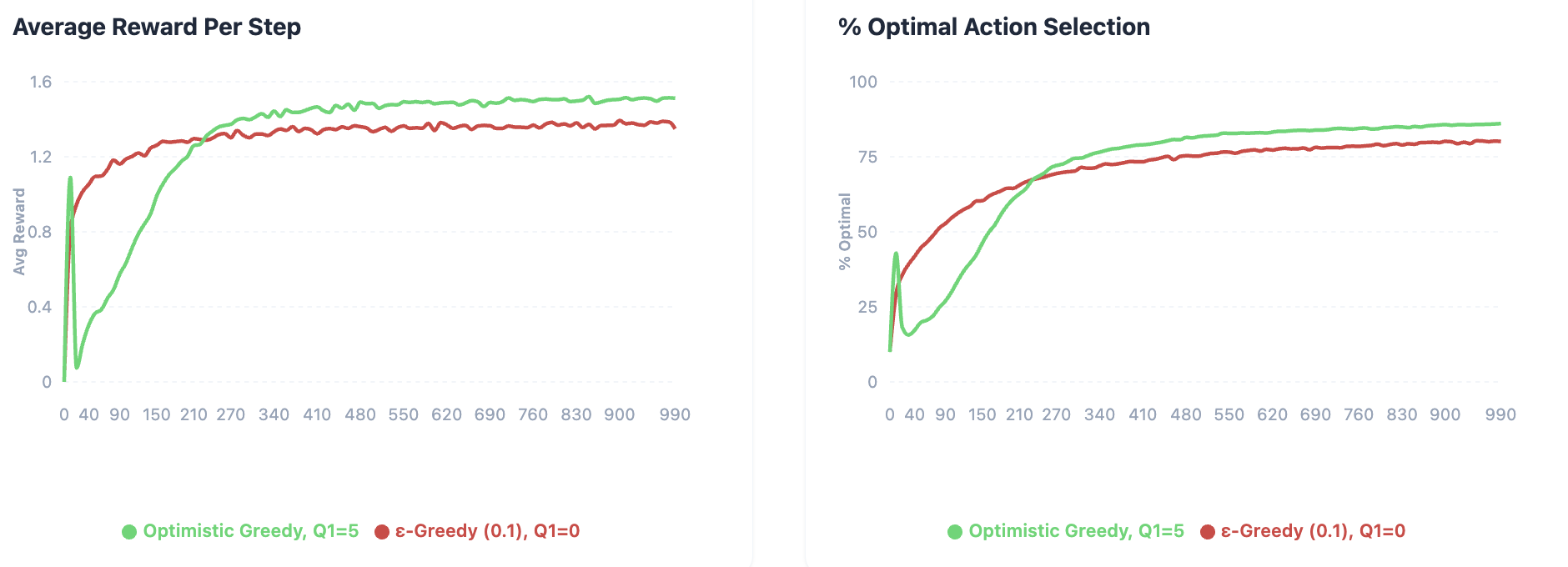Optimistic Initial Values Comparison between ϵ-greedy and greedy with optimistic initial values. Notice a spike for optimistic greedy in the begining? why and where it could be occuring?

Smarter Exploration with Upper Confidence Bounds (UCB)

ϵ-greedy selects non-greedy actions randomly from the set of non-optimal actions but it doesn't give any preference to any nearly greedy or uncertain actions. Attaching a metric to actually assess the potential of an action to actually be optimal is the key idea behind Upper Confidence Bounds (UCB). UCB take into account the uncertainty of the action-value estimates and the closeness of their estimates for being optimal. UCB selects actions based on the following metric:

A_t = \arg\max_{a} [Q_t(a) + c\sqrt{\frac{ \ln t}{N_t(a)}}]

$N_t(a)$ is the number of times action $a$ has been selected up to time $t$ . $c$ is a constant that controls the amount of exploration. The square root term is a measure of uncertainty of the action-value estimate. The overall term is a measure of upper bound of the action value estimate where $c$ kind of determines the confident level. The amount of uncertaainity decreases as the number of times an action is selected increases (the square root term is a quantified measure that explains this relationship).

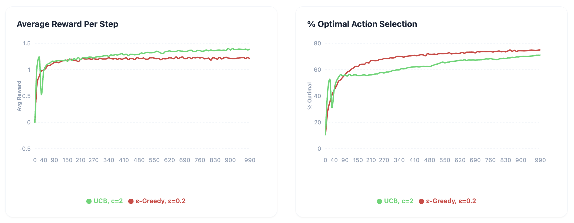UCB Comparison between ϵ-greedy and UCB. Notice how the average reward is higher for UCB despite having lesser optimal actions selected? what could be the reason for the spike at the begining of UCB and where exactly it is occuring?

Gradient Bandits: Learning Preferences for Actions

All the methods that we discussed so far are using action-value estimates to select actions. Is there any way to disassociate the action selection criteria from action-value estimates? Gradient bandit algorithm does this to some extent by giving numerical preferences to every action. Let $H_t(a)$ be the preference for action $a$ at time $t$ . The probability $\pi_t(a)$ of selecting action $a$ is given by

\pi_t(a) = \frac{e^{H_t(a)}}{\sum_{b=1}^{A} e^{H_t(b)}}

The preferences $H_t(a)$ are updated based on the rewards received. The update rule is given by

H_{t+1}(a) = H_t(a) + \alpha [R_t - \bar{R}_t]\pi_t(a) \quad \text{if } a \neq A_t \\ H_{t+1}(A_t) = H_t(A_t) + \alpha [R_t - \bar{R}_t](1 - \pi_t(A_t)) \quad \text{if } a = A_t

Here $\bar{R}_t$ is the average reward of all actions up to time $t$ . $\bar{R}_t$ is used as a baseline to compare the reward of the current action with the average reward of all actions thereby deciding whether to increase or decrease the preference for the current action. $\alpha$ is the step size parameter. These update rules and probability calculation criterion are pretty common in Deep Learning to train neural networks.

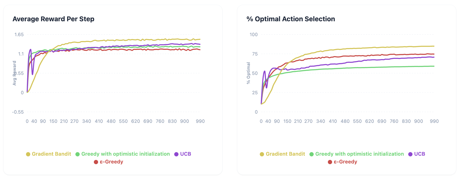Gradient Bandits Comparison of all the methods discussed so far.

Interactive Demo

Try out the interactive demo below to get a better understanding of how these algorithms work. You can change the parameters of the algorithms, compare them side by side and see how they perform on any k-armed bandit testbed you can think of with different reward distributions.

ϵ-Greedy: Balance exploration and exploitation with the ϵ parameter.
UCB (Upper Confidence Bound): Explore actions with high uncertainty using the confidence parameter.
Gradient Bandit: Learn action preferences using gradient-based updates.
Optimistic Initial Values: Set high initial Q-values to encourage early exploration.

Interactive labChange inputs · observe results

Loading interactive lab…

References

Sutton, R. S., & Barto, A. G. (2018). Reinforcement Learning: An Introduction.

Tools

Image Generation: Gemini, ChatGPT
Interactive Demo: Google AI Studio
Editor: Antigravity