Monte Carlo Methods - Learning from Experience

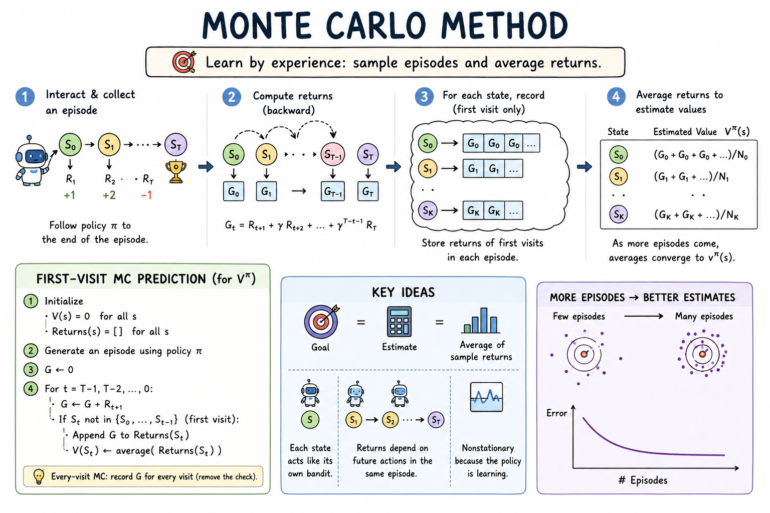
An illustration of Monte Carlo Methods

This post captures my takeaways from Chapter 5 of the book Reinforcement Learning: An Introduction by Sutton and Barto, the bible of RL.

Core Idea and Prior Knowledge

Monte Carlo (MC) methods are a class of learning algorithms that estimate value functions and discover optimal policies directly from raw experience. By relying on sequences of states, actions, and rewards, MC methods eliminate the need for a complete model of the environment's dynamics. This makes them exceptionally well-suited for complex, real-world problems where state transition probabilities are unknown, but interaction either through physical experience or simulation is possible. Unlike Dynamic Programming, which requires a perfect model to compute values, Monte Carlo methods learn simply by averaging the returns observed in actual trajectories.

Critically, these methods rely on episodic experience. Interaction is divided into discrete episodes, sequences that transition from an initial state to a terminal one. This structure ensures that every state encountered has a well-defined return, allowing the agent to refine its policy and value estimates incrementally after each episode’s conclusion.

Conceptually, MC's averaging of returns is an extension of the techniques explored in Multi-Armed Bandits, with the key difference being that MC must navigate multiple states, essentially treating each state as a distinct bandit problem. While bandit rewards are immediate and independent, MC returns are interconnected. The total return received after a visit to an earlier state depends on every action taken in subsequent states within that same episode. Because the agent is simultaneously learning and updating its policy for those later states, the distribution of future returns for earlier states is constantly shifting. From the perspective of an early state, its "reward distribution" appears non-stationary, as the eventual reward depends on a policy that is being continuously optimized through experience.

General Policy Iteration (GPI) from the DP is used here for MC methods to handle non-stationary nature of the problem. While we computed value functions from the knowledge of MDP, here we learn value function from sample returns with MDP.

The Experience : Monte Carlo Prediction

We start with learning state-value function ($v_\pi(s)$), the expected returns (expected cumulative future rewards) from states assuming some policy. The simplest way to estimate the value of a state under a policy is to average returns from many visits to that state which converges to true value as number of visits increases.

Each state can be visited multiple times in an episode. Based on this occurence criteria, we have two types of MC methods:

• First-visit MC: For each state, we average returns following the first visit to that state in an episode.
• Every-visit MC: For each state, we average returns following every visit to that state in an episode.

Both of them converge to the true value function as the number of visits to each state goes to infinity.

def first_visit_mc(env, policy, num_episodes):
    V = defaultdict(float)        # state-value function
    returns_sum = defaultdict(float)  # sum of returns
    N = defaultdict(int)          # number of visits
    
    for _ in range(num_episodes):
        G = 0
        episode = []
        
        S, _ = env.reset()
        state_visited = False
        
        while not env.is_done(S):
            A = policy(S)
            next_S, R, done = env.step(A)
            
            episode.append((S, R))
            G += R
            
            if not state_visited:
                returns_sum[S] += G
                N[S] += 1
                state_visited = True
            
            S = next_S
        
        # Update value function
        for s, _ in episode:
            V[s] = returns_sum[s] / N[s]
            
    return V

def every_visit_mc(env, policy, num_episodes):
    V = defaultdict(float)        # state-value function
    returns_sum = defaultdict(float)  # sum of returns
    N = defaultdict(int)          # number of visits
    
    for _ in range(num_episodes):
        G = 0
        episode = []
        
        S, _ = env.reset()
        
        while not env.is_done(S):
            A = policy(S)
            next_S, R, done = env.step(A)
            
            episode.append((S, R))
            G += R
            
            returns_sum[S] += G
            N[S] += 1
            
            S = next_S
        
        # Update value function for all visits
        for s, _ in episode:
            V[s] = returns_sum[s] / N[s]
            
    return V

The Search : Estimating Action-Values

As we discussed in Idea section that a perfect model is not required for MC methods, we solve the problem of finding optimal policy without any model by finding optimal action-value function $q_*$. The policy evaluation problem for action-value is to estimate $q_\pi(s,a)$ (expected return for taking action $a$ from state $s$ following policy $\pi$). A state-action pair is said to be visited if action $a$ has ever been taken from state $s$.

A lot of times there can be many state-action pairs which will never be visited, especially for cases of deterministic policy where there is always one action chosen from a given state. Exploring starts is introduced to overcome this limitation by ensuring every pair has non-zero probability of being selected as the start of an episode. One other alternative to ensure that all state-action pairs are visited is to use stochastic policies with non-zero probability of selecting all actions from a given state.

The Loop : Monte Carlo Control

Let's re-visit the concept of General Policy Iteration (GPI) from the DP section. At high-level, GPI maintains approximate policy and approximate value function. The value function is updated [policy evaluation] to approximate value function for current policy while policy is repeatedly improved [policy improvement] wrto current value function.

Policy evaluation has already been discussed in the previous section. Policy improvement is done by making the policy greedy wrto current value function. (as shown in equation below).

To avoid the assumption of infinite number of episodes for convergence, let's recap the approaches that are discussed in DP.

• Approximating $q_{\pi_k}$: We bound the magnitude and probability of estimation errors, repeating policy evaluation steps until these bounds become negligible.
• Partial Policy Evaluation: Instead of repeating policy evaluation steps until convergence, we perform policy evaluation for a fixed number of steps.
• Value Iteration: One iteration of policy evaluation is performed after every policy improvement step.

Incase of Monto Carlo, we alternate b/w evaluation and improvement on a episode by episode basis i.e., during policy evaluation, policy is improved at all states that are visited during the episode. The algorithm is called Monto Carlo ES (ES stands for Exploring Starts).

def mc_es(env, num_episodes):
    Q, returns, N = defaultdict(float), defaultdict(float), defaultdict(int)
    policy = defaultdict(lambda: np.random.choice(env.action_space.n))
    
    for _ in range(num_episodes):
        S, _ = env.reset()  # exploring starts
        episode = []
        
        while not env.is_done(S):
            A = policy[S]
            next_S, R, _ = env.step(A)
            episode.append((S, A, R))
            S = next_S
            
        G = 0
        for S, A, R in reversed(episode):
            G += R
            returns[S, A] += G
            N[S, A] += 1
            Q[S, A] = returns[S, A] / N[S, A]
            policy[S] = max(range(env.action_space.n), key=lambda a: Q[S, a])
            
    return Q, policy

How to avoid exploring starts?

One of the assumptions during the formulation of Monto Carlo Control is that exploring starts are allowed, i.e. for every state-action pair $(s, a)$ there is non-zero probability that the pair can be selected as the start of the episode. To avoid this assumption and ansure all the actions are selected, we have two methods: On-policy and Off-policy methods.

On-policy Method

On-policy method evaluates and improves the same policy used for making decisions. Monte Carlo ES is an on-policy method. The policy starts as soft policy (i.e. $\pi(a|s) > 0$ for all $s,a$) and gradually becomes determenistic. We use a $\epsilon$-greedy policy to ensure that all state-action pairs are visited. In $\epsilon$-greedy policy, all non-greedy actions are given a minimal probability $\epsilon/|\mathcal{A}|$ of being selected, ensuring continuous exploration while a probability of $1-\epsilon + \epsilon/|\mathcal{A}|$ is given to the greedy action. Note that this on-policy MC control is still a GPI. For any $\epsilon$-soft policy $\pi$, any $\epsilon$-greedy policy is always better than or equal to $\pi$.

def on_policy_mc_control(env, num_episodes, epsilon):
    Q, returns, N = defaultdict(float), defaultdict(list), defaultdict(int)
    n_actions = env.action_space.n
    # Initialize ε-soft policy: uniform probabilities
    policy = defaultdict(lambda: np.ones(n_actions) / n_actions)

    for _ in range(num_episodes):
        # Generate episode following π
        episode = []
        S, _ = env.reset()
        while not env.is_done(S):
            A = np.random.choice(n_actions, p=policy[S])
            next_S, R, _ = env.step(A)
            episode.append((S, A, R))
            S = next_S

        G = 0
        visited = set()
        for S, A, R in reversed(episode):
            G += R
            if (S, A) not in visited:  # first-visit check
                visited.add((S, A))
                returns[S, A].append(G)
                Q[S, A] = np.mean(returns[S, A])
                A_star = max(range(n_actions), key=lambda a: Q[S, a])
                for a in range(n_actions):
                    policy[S][a] = 1 - epsilon + epsilon / n_actions if a == A_star else epsilon / n_actions

    return Q, policy

A good task here would be to prove that for any $\epsilon$-soft policy $\pi$, any $\epsilon$-greedy policy is always better than or equal to $\pi$.

Off-policy Method

Off-policy methods allow the agent to evaluate and improve policies different from the one used for action selection. The policy that is being learnt and becomes optimal poliocy is called Target policy. The policy that is exploratiory and used to generate behaviour is called Behaviour policy (Off because the learning comes from data which is "off" the target policy).

Off-policy methods are generally of higher variance and converges slowly compared to on-policy methods. Off-policy methods are more powerful and even includes On-polcy method as a special case. Off-policy can be applied in areas where we have data generated by human experts or from a controller.

Let's start with a problem where both target abd behavior policies are fixed making it a prediction problem. All the episodes are following behavior policy $b$ different from target policy $\pi$ used for estimating $v_\pi$ or $q_\pi$. For Off-policy to work, we need every action take under $\pi$ should also be taken under $b$ (referred to as assumption of coverage). $b$ must also be stochastic in states where it's not identical to $\pi$. While there is no condition on $\pi$, we would like it to be deterministic so as to utilize in control applications.

Target policy is deterministic greedy policy (ideal but not necessary) while Behavior policy is stochastic and more exploratory.

Importance Sampling is a method for evaluating particular target distribution while using samples from a different distribution. I reccommend going through this blog to understand more about this topic. A term importance sampling ratio, defined as ration of trajectories from target and behavior policy is introduced in-order to estimate $\pi$. Let use assume a trajectory: $A_t \xrightarrow{} S_{t+1} \xrightarrow{} A_{t+1} \xrightarrow{} S_{t+2} \dots \xrightarrow{} A_{T-1} \xrightarrow{} S_T$ where $T$ is the terminal time step. The importance sampling ratio for this trajectory is defined as:

This ratio can be used to determine $v_\pi(s)$ from returns $gG_t$ observed from behavior policy $b$ as shown in the equation below:

Let $T(s)$ be the set of time steps in the episodes where $s$ is visited (first visit). Finally to estimate $v_\pi(s)$, returns from $b(s)$ are scaled and averaged using importance sampling ration in two ways:

• Ordinary Importance Sampling: Returns are weighted by importance sampling ratio and then averaged. This method is unbiased but has unbounded variance.

• Weighted Importance Sampling: Returns are weighted by importance sampling ratio and then normalized by the sum of the ratios. This method is biased but has lower variance and connverges to zero for bounded returns. Due to it's lower variance, this method is strongly preferred in practice.

The unbounded variance effects especially for trajectories that contains loops causing infinite variance.

The Efficiency : Incremental Implementation

In Multi armed bandits, we have used incremental implementation to average rewards efficiently without storing all the rewards. Similar method can be used both for on-policy and off-policy methods to average returns.

Ordinary importance sampling can directly utilize equantions from Multi armed bandits:

For weighted importance sampling we need to track weighted average of returns. Let $W_i = \rho_{t:T-1}$ and $G_1, G_2, \dots G_n$ are sequence of returns and $C_n$ be cummulative sum of weights for the first $n$ returns. Then the incremental implementation can be derived as shown below:

def off_policy_mc_control(env, num_episodes):
    Q, C = defaultdict(float), defaultdict(float)
    target_policy = defaultdict(lambda: np.random.choice(env.action_space.n))
    behavior_policy = defaultdict(lambda: np.random.choice(env.action_space.n))

    for _ in range(num_episodes):
        S, _ = env.reset()
        episode = []
        
        while not env.is_done(S):
            A = behavior_policy[S]
            next_S, R, _ = env.step(A)
            episode.append((S, A, R))
            S = next_S
            
        G = 0
        W = 1
        
        for S, A, R in reversed(episode):
            G += R
            C[S, A] += W
            Q[S, A] += (W / C[S, A]) * (G - Q[S, A])
            target_policy[S] = max(range(env.action_space.n), key=lambda a: Q[S, a])
            
            if A != target_policy[S]:
                break
            
            W *= 1 / behavior_policy[S][A]

Off-Policy Monte Carlo Control

The final pseudocde for Off-policy Monte Carlo Control is shown below. The target policy is updated to be greedy wrto current action-value function while behavior policy is fixed and more exploratory.

def off_policy_mc_control(env, num_episodes):
    Q, C = defaultdict(float), defaultdict(float)
    target_policy = defaultdict(lambda: np.random.choice(env.action_space.n))
    behavior_policy = defaultdict(lambda: np.random.choice(env.action_space.n))

    for _ in range(num_episodes):
        S, _ = env.reset()
        episode = []

        while not env.is_done(S):
            A = behavior_policy[S]
            next_S, R, _ = env.step(A)
            episode.append((S, A, R))
            S = next_S

        G = 0
        W = 1

        for S, A, R in reversed(episode):
            G += R
            C[S, A] += W
            Q[S, A] += (W / C[S, A]) * (G - Q[S, A])
            target_policy[S] = max(range(env.action_space.n), key=lambda a: Q[S, a])

            if A != target_policy[S]:
                break

            W *= 1 / behavior_policy[S][A]

Off-policy weighted importance sampling learns only from tails of episodes when the actions prior it are greedy. On the other hand if non-greedy actions are common, then the learning is slower considering higher % of disagreements b/w target and behavior policies (non-greedy actions).

Example : The Game of Blackjack

Blackjack is a popular casino card game where a player competes independently against a dealer. The fundamental objective is to obtain cards whose numerical sum is as great as possible without exceeding 21. All face cards (Jack, Queen, King) are worth 10 points, while Aces are worth either 1 or 11 points.

If you're not familiar with the game of Blackjack, I recommend watching this video which explains the rules well.

Gameplay

• The Deal: The game begins with two cards dealt to both the dealer and the player. One of the dealer's cards is face up, and the other is face down.

• The Natural: If the player hits a sum of 21 immediately (i.e, an Ace and a 10-value card), it is called a Natural. The player wins automatically unless the dealer also has a natural, which results in a draw (a push).

• The Player's Decisions: If no one has a natural, the player makes one by one choices to optimize their hand. At each turn, they can perform one of these actions:

  • Hit: The player requests an additional card to increase their cumulative sum. They can continue hitting until they decide to stop or until their sum exceeds 21 (known as going bust, which results in an immediate loss).

  • Stick: The player chooses to stop receiving cards and freezes their current total. This immediately concludes their turn, locks in their final score, and officially passes play to the dealer.

• The Dealer's Turn: Once the player concludes their turn by sticking, the dealer plays out their hand. Unlike the player, the dealer has zero autonomy and must follow a strict, predictable rule: they must stick on any sum of 17 or greater, and hit otherwise.

• The Outcome: If the dealer goes bust, the player wins. Otherwise, the final card sums of the player and dealer are compared—whoever's final sum is closer to 21 without exceeding it wins the game. If their final scores are identical, the game is a draw.

Framing the Game as an RL Problem

Blackjack is a classic example of episodic finite MDP where each game is an episode.

• Rewards of +1, -1, 0 are given for win, loss and draw respectively. The player's actions are either to hit or stick.

• State Space : The player makes decisions based on three specific variables, creating a total of 200 distinct states.

1. Player's Current Sum (12–21): Sums from 2 to 11 are omitted from the decision state space because a player cannot go bust on these totals and should obviously always choose to hit.

2. Dealer's Showing Card (Ace–10): The single card the dealer displays face up.

3. Usable Ace (True/False): An Ace is considered "usable" if the player can count it as 11 without going bust. If counting it as 11 would push the sum over 21, it is automatically counted as a 1 and is no longer usable.

Interactive Demo

Below is an interactive Monte Carlo Blackjack Visualizer. It allows you to run Monte Carlo algorithms in real-time and lets you easily switch between five distinct approaches:

1. First-Visit MC
2. Every-Visit MC
3. Monte Carlo ES
4. ε-Greedy (with an adjustable exploration rate)
5. Off-Policy learning

Visualizer provides three real-time lenses into its learning process:

1. The Live Table: Watch individual episodes unfold step-by-step, seeing the exact card draws, player sum, dealer showing card, and the final reward.
2. Value & Policy Functions: Watch the agent's "brain" update live. You can toggle between rich 3D Surface Plots and crisp 2D Heatmaps to interpret the learned State-Value Function ($V$) and Policy ($\pi$) across both Usable Ace and No Usable Ace states.
3. Trajectory Flow Graph: A visual web of decisions tracking the recent paths (states and actions) the agent has taken. Thicker lines reveal the most frequently sampled paths ending in a Hit, Stick, or Bust.

References

1. Sutton, R. S., & Barto, A. G. (2018). Reinforcement Learning: An Introduction.
2. Liu, J. Importance Sampling Explained End-to-End. https://medium.com/@liuec.jessica2000/importance-sampling-explained-end-to-end-a53334cb330b

Tools

• Image Generation: ChatGPT
• Editor: Antigravity
• Interactive Demo: Google AI Studio