
DotChat Demo
This blog assumes you have a basic understanding of LLMs and how they're trained. If not, I would recommend you to first go through this llm-course by Maxime Labonne.
Why DotLM?
Last time I wrote a blog post (about the STE Dataset), OpenClaw was trending. Now, as I write this, Andrej Karpathy's "LLM Knowledge Bases" concept is the latest focus. People are finding innovative ways to integrate LLMs into their daily workflows; I personally use Claude Code for many of my projects, both personal and professional. It’s remarkable to see what these models are capable of, and they only continue to improve. Anthropic's latest internal model, Mythos, is particularly mind-blowing, while not yet public, its reported capabilities are incredible and dangerous.
LLM Knowledge Bases
— Andrej Karpathy (@karpathy) April 2, 2026
Something I'm finding very useful recently: using LLMs to build personal knowledge bases for various topics of research interest. In this way, a large fraction of my recent token throughput is going less into manipulating code, and more into manipulating…
As I mentioned in my previous blog post, I have always been fascinated by how a set of matrices can be trained to almost replace an entry-level software engineer. As an ML researcher, I understand the mathematics behind them, still it amazes me how they work. Few years back I wouldn't have imagined that a Language model would be able to do so much and has capabilities to even solve un-solved Maths and Physics problems (GPT-5.4 cracked a 20 year old Maths problem). This led me to build a miniature version of it myself from the ground up. This led me to develop a tiny, reasoning-capable language model—often referred to as an SLM (Small Language Model).
If you're also interested in training an LLM from scratch, I highly recommend the Smol Training Playbook from Hugging Face.
Dataset
There are plenty of open-source datasets like FineWeb, Wikipedia, and RedPajama that are perfect for pretraining. Since my objective was to train a reasoning-capable model (a characteristic usually reserved for much larger systems) using fewer parameters, I needed a high information density dataset. Extensive research on existing datasets and their composition led me to create my own STE dataset, covering all four stages of LLM training. The synthetic data focuses on core concepts across various domains like Physics, Chemistry, Biology, Mathematics, Computer Science, and General Knowledge. I also added few samples from FineWeb, Wikipedia to the pretraining dataset (only because I haven't generated enough pretraining tokens).
Samples from STE Dataset
Pretraining Sample
In case of Reasoning, thought_trace and output responses were compressed using gpt-4o-mini as the original responses were too long.
DotLM Architecture
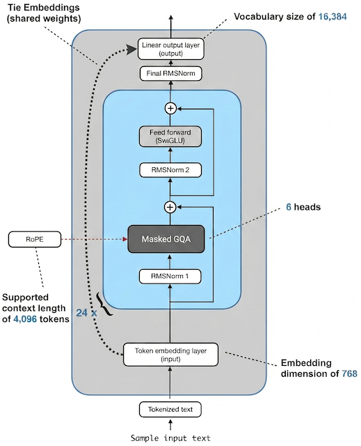 DotLM Architecture
Illustration inspired from Sebastian Raschka's LLM Gallery
The DotLM architecture is a decoder-only transformer inspired by Qwen 3. While key components like SwiGLU, RMSNorm, RoPE, and GQA are borrowed from Qwen 3, several architectural modifications were introduced to enable reasoning at a 165M parameter scale. My selection process focused on parameter-efficient components to minimize the model's size.
Specs
| Configuration | Value |
|---|---|
| Total Parameters | 165,342,720 (~165M) |
| Layers | 24 |
| 768 | |
| (Intermediate Dim) | 2,048 (2.67x ratio) |
| Attention Heads | 6 |
| KV Heads | 2 (Grouped Query Attention) |
| Head Dimension | 128 |
| Context Length | 4,096 |
| Tokenizer | BPE |
| Vocabulary Size | 16,384 |
| Activation Function (FeedForward) | SwiGLU |
| Normalization | RMSNorm () |
| Positional Embedding | RoPE () |
| Weight Tying | Enabled (Input/Output Embeddings) |
| Training Precision | BF16 Mixed |
The optimal configuration was determined through hyperparameter tuning using Autoresearch (detailed later in this post).
Grouped Query Attention (GQA)
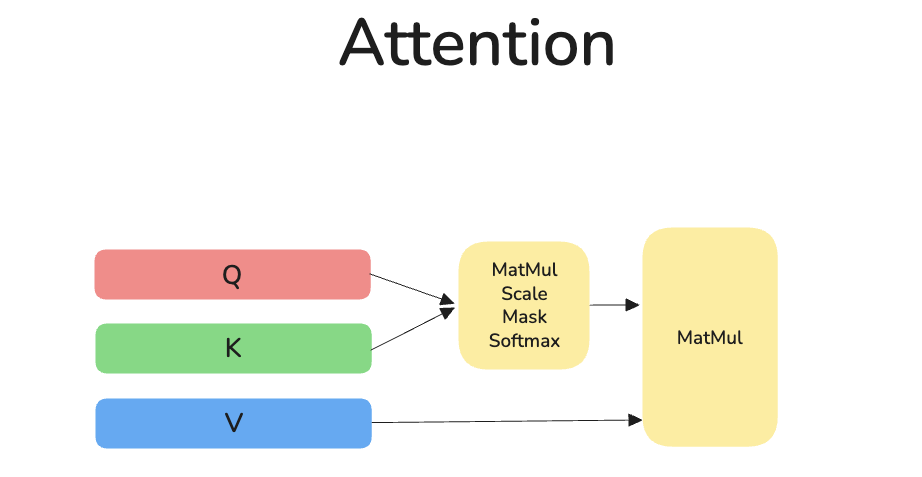
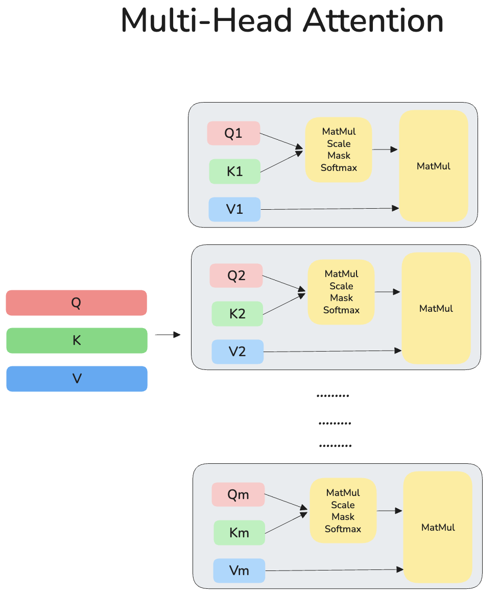
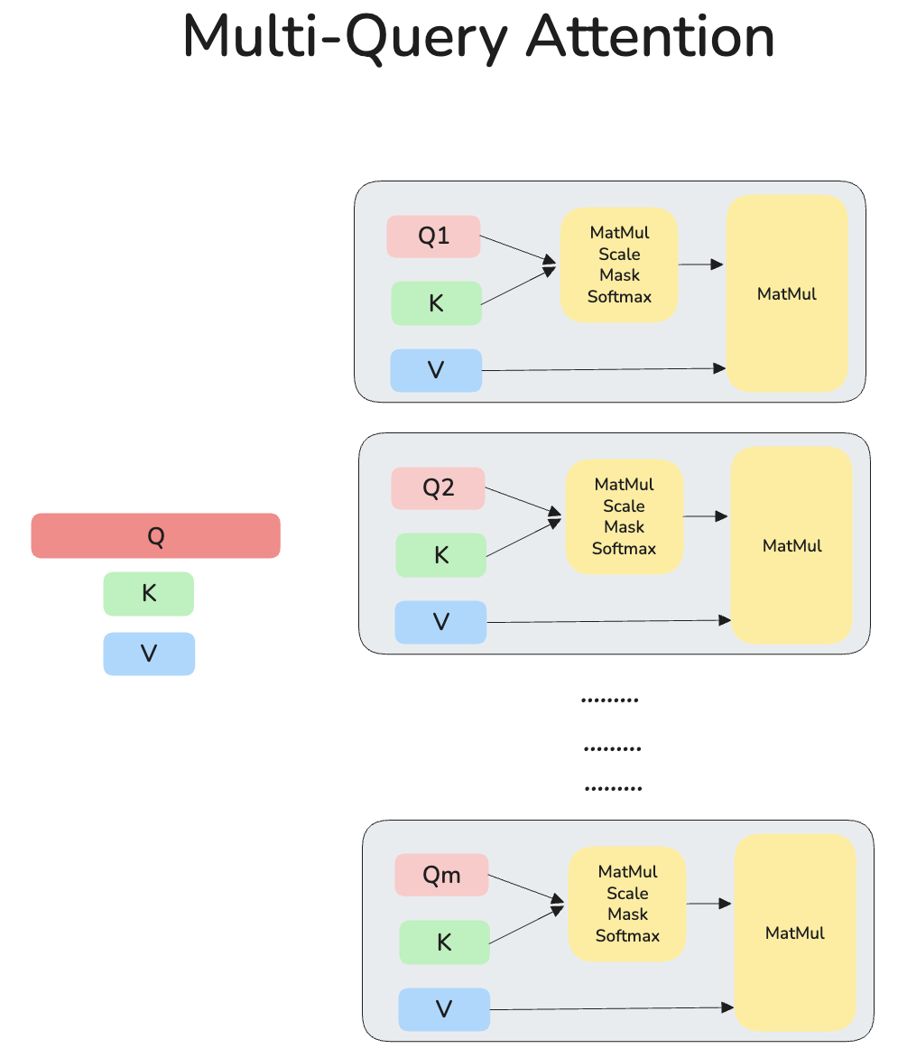
Grouped Query Attention (GQA) bridges the gap between Multi-Head Attention (MHA) and Multi-Query Attention (MQA) by grouping query heads to share a single key-value head. This significantly reduces the memory bandwidth required for the KV cache during inference while maintaining quality close to MHA. In MHA, we have query, key, and value heads. In GQA, we have query heads but only key/value heads ().
Special cases of GQA are:
- Multi-Head Attention (MHA):
- Multi-Query Attention (MQA):
 Attention
 Multi-Head Attention
 Multi-Query Attention
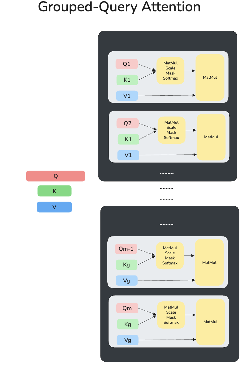 Grouped-Query Attention
Attention
SwiGLU
SwiGLU is an activation function that combines the SWISH (or SiLU) activation with a Gated Linear Unit (GLU). It has been empirically shown to offer better performance than standard ReLU or GeLU. It dynamically gates the flow of information using a learned linear projection passed through a Swish function.
RMSNorm
Root Mean Square Normalization (RMSNorm) is a simpler and faster alternative to standard Layer Normalization. It removes the mean-centering step, hypothesizing that the scaling invariance is the most important component of LayerNorm's success. This reduces computational overhead while maintaining training stability.
where is the input vector of dimension , is a small constant for numerical stability, and is a learned scale parameter.
Tie Embeddings
Weight tying shares the parameters between the token embedding layer and the language modeling head (pre-softmax projection). This reduces the total parameter count by reusing the learned linguistic representations for both mapping tokens to vectors and vectors back to logits.
Rotary Positional Embeddings (RoPE)
RoPE encodes positional information by rotating the queries and keys in the complex plane, rather than adding an absolute positional vector. This preserves relative distances and provides better extrapolation capabilities for longer context windows. For a given position and a 2D feature vector , it applies the rotation matrix:
For higher dimensions, it pairs consecutive dimensions and rotates each pair with different frequencies .
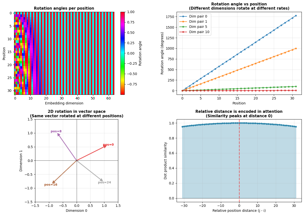 Rotary Positional Embedding Analysis
Autoresearch
As its name suggests, Autoresearch is a framework designed to automate hyperparameter tuning for neural networks using AI agents. This concept was proposed by Andrej Karpathy in a recent X post. The primary advantage of Autoresearch over traditional methods (such as Grid Search or Bayesian Optimization) is its ability to perform unstructured, autonomous code evolution rather than merely searching within a predefined parameter space. This gives researchers greater control over design criteria and the ability to discover novel architectural patterns.
The idea: give an AI agent a small but real LLM training setup and let it experiment autonomously overnight. It modifies the code, trains for 5 minutes, checks if the result improved, keeps or discards, and repeats.
I packaged up the "autoresearch" project into a new self-contained minimal repo if people would like to play over the weekend. It's basically nanochat LLM training core stripped down to a single-GPU, one file version of ~630 lines of code, then:
— Andrej Karpathy (@karpathy) March 7, 2026
- the human iterates on the… pic.twitter.com/3tyOq2P9c6
Workflow
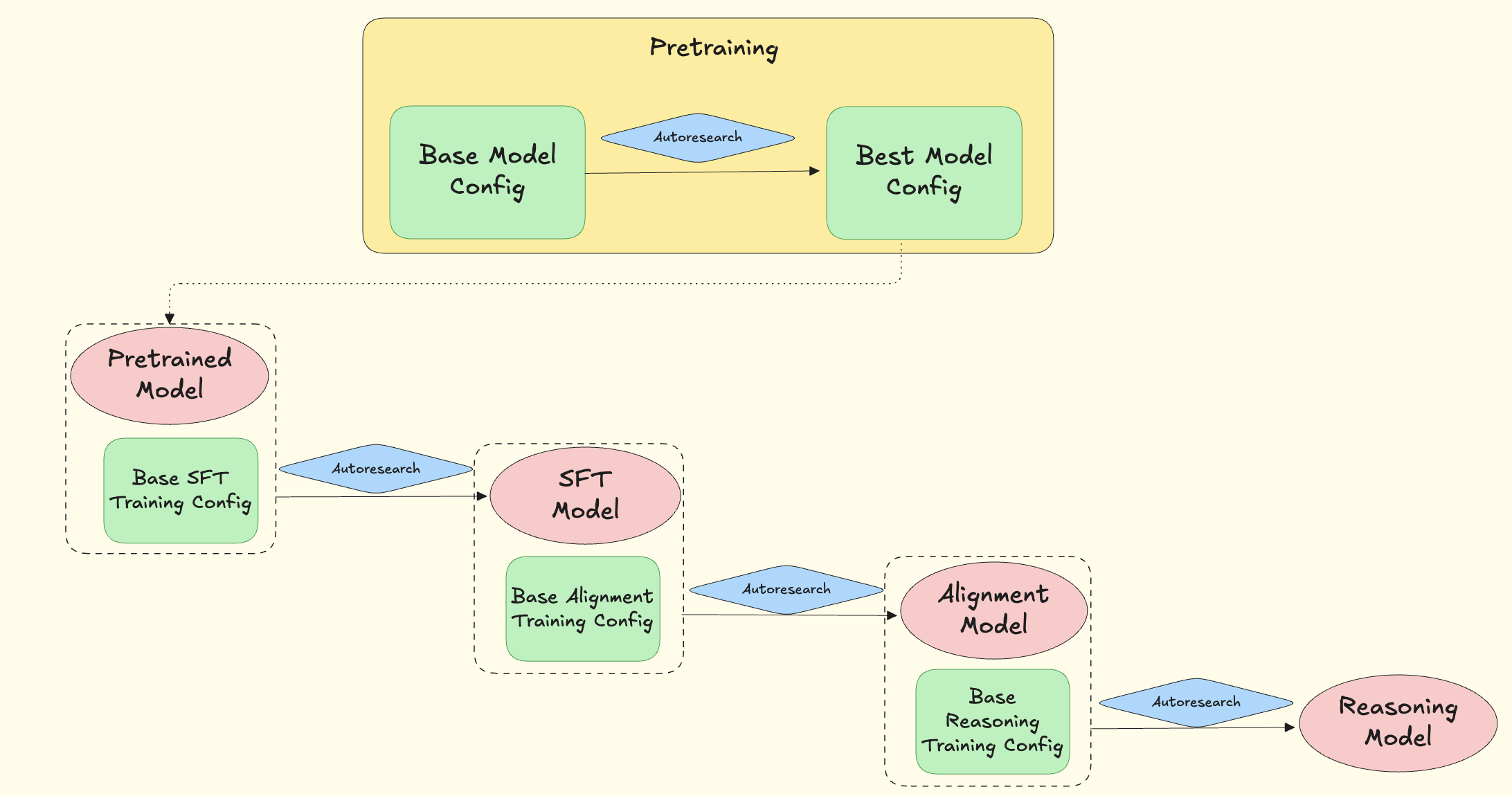 DotLM Training Workflow using Autoresearch
We start with a base configuration file and a pretraining dataset. Autoresearch optimizes architecture settings to identify the best model, which is then used to train subsequent stages: SFT, Alignment, and Reasoning. In these later stages, Autoresearch is used to optimize training settings. While validation loss is the primary metric for parameter tuning, the agent also evaluates the quality of generated samples to ensure the model is learning meaningful patterns (a predefined set of 20 prompts is used for these quality checks).
Pretraining - Knowledge Acquisition
Pretraining is the most critical, resource-intensive, and time-consuming stage of training an LLM. During this phase, the model learns about language, facts, and the world. Once trained, the model functions as an auto-complete engine, predicting the next token based on previous sequences.
Using approximately 246M tokens from the STE pretraining dataset, the model was trained for 10 epochs (totaling ~2.46B tokens), which aligns with Chinchilla optimality for a 165M parameter model. The hyperparameters optimized were:
- Model Architecture
- Max Sequence Length
- Hidden Dim
- Attention Heads
- KV Heads
- RoPE
theta - Num layers
- Training Hyperparameters
- Batch Size + Accumulation
- Learning Rate
- WSD scheduler (Warmup-Stable-Decay) settings
- Gradient Clipping
Beta1,Beta2for AdamW optimizer
| Hyperparameter | Value |
|---|---|
| Dataset | 352k samples (~246M tokens) |
| Training Tokens | ~2.46B (10 Epochs) |
| Total Steps | ~27,500 Optimizer Steps |
| Batch Size | 64 (Accum=2, Effective=128) |
| Learning Rate | |
| Weight Decay | 0.01 |
| Scheduler | WSD (Warmup-Stable-Decay) |
| Warmup Steps | 2,750 (~10%) |
| Stable Steps | 20,000 (~73%) |
| Decay Steps | 4,750 (~17%) |
| Gradient Clipping | 0.5 |
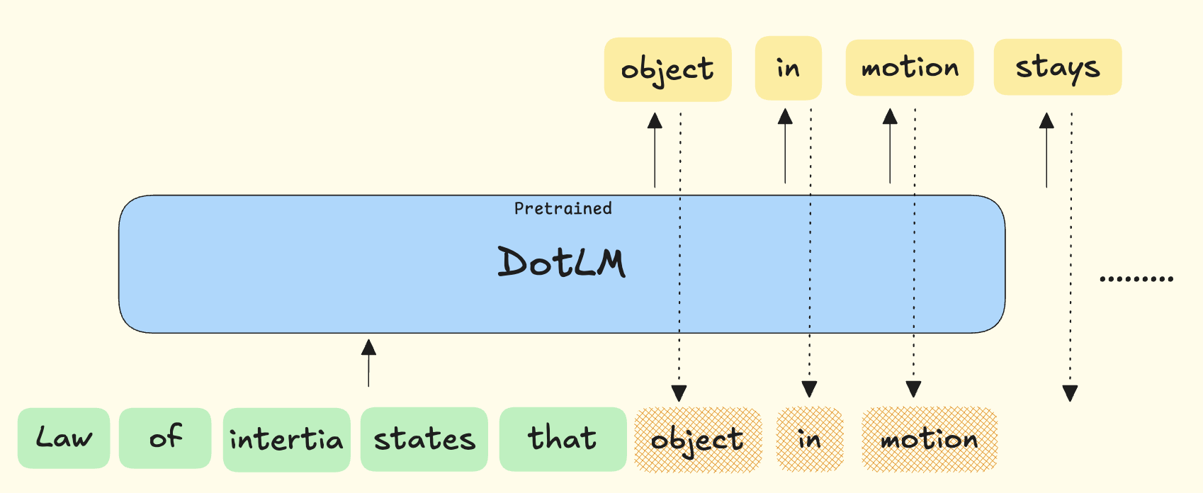 Sample text generation after Pretraining
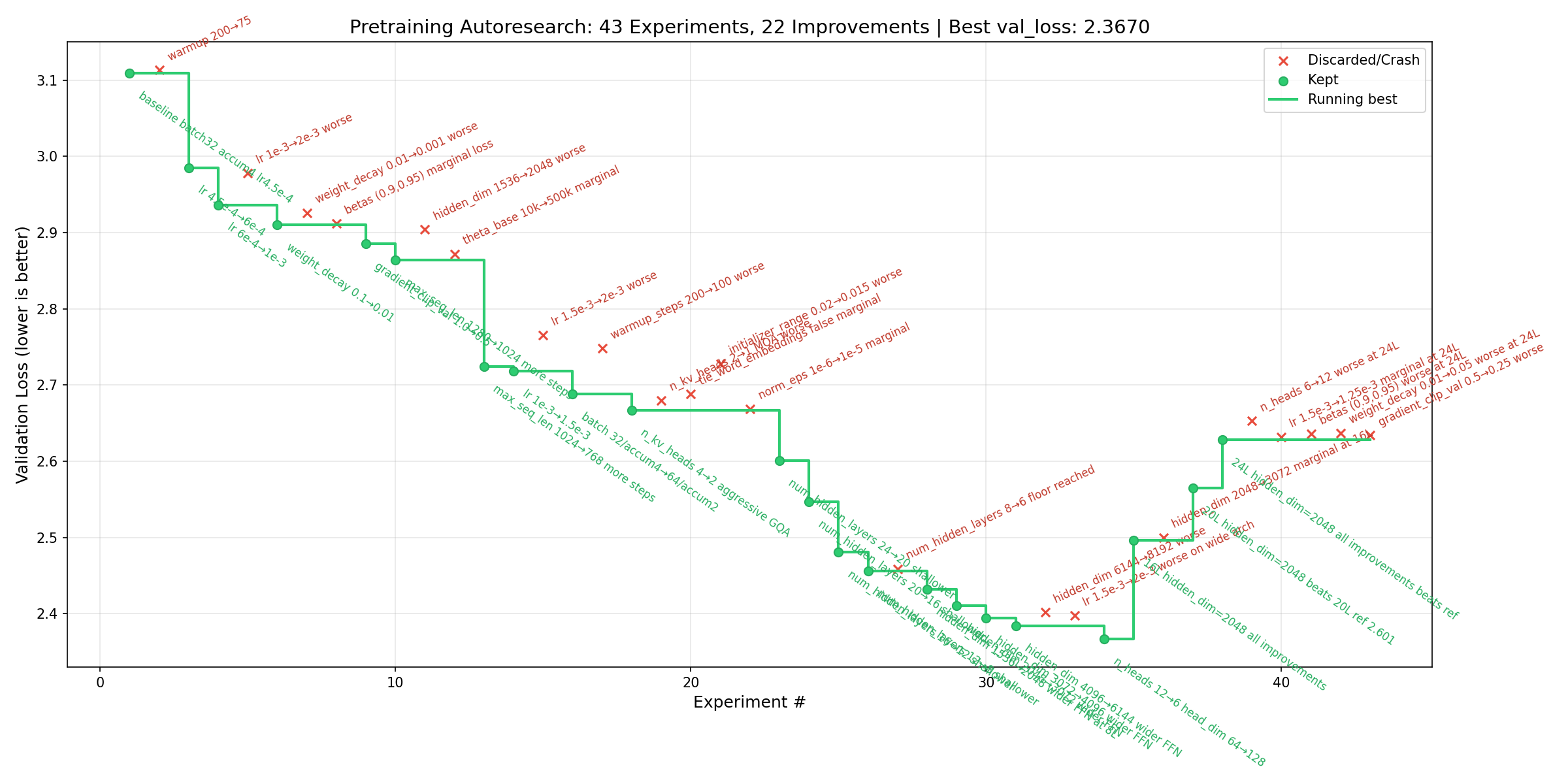 Autoresearch progress during Pretraining
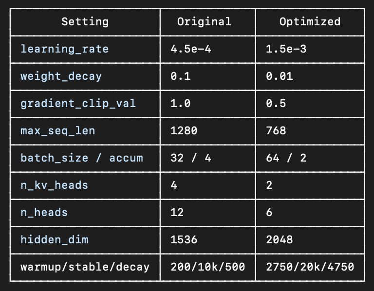 Changes in architecture and training settings during Pretraining
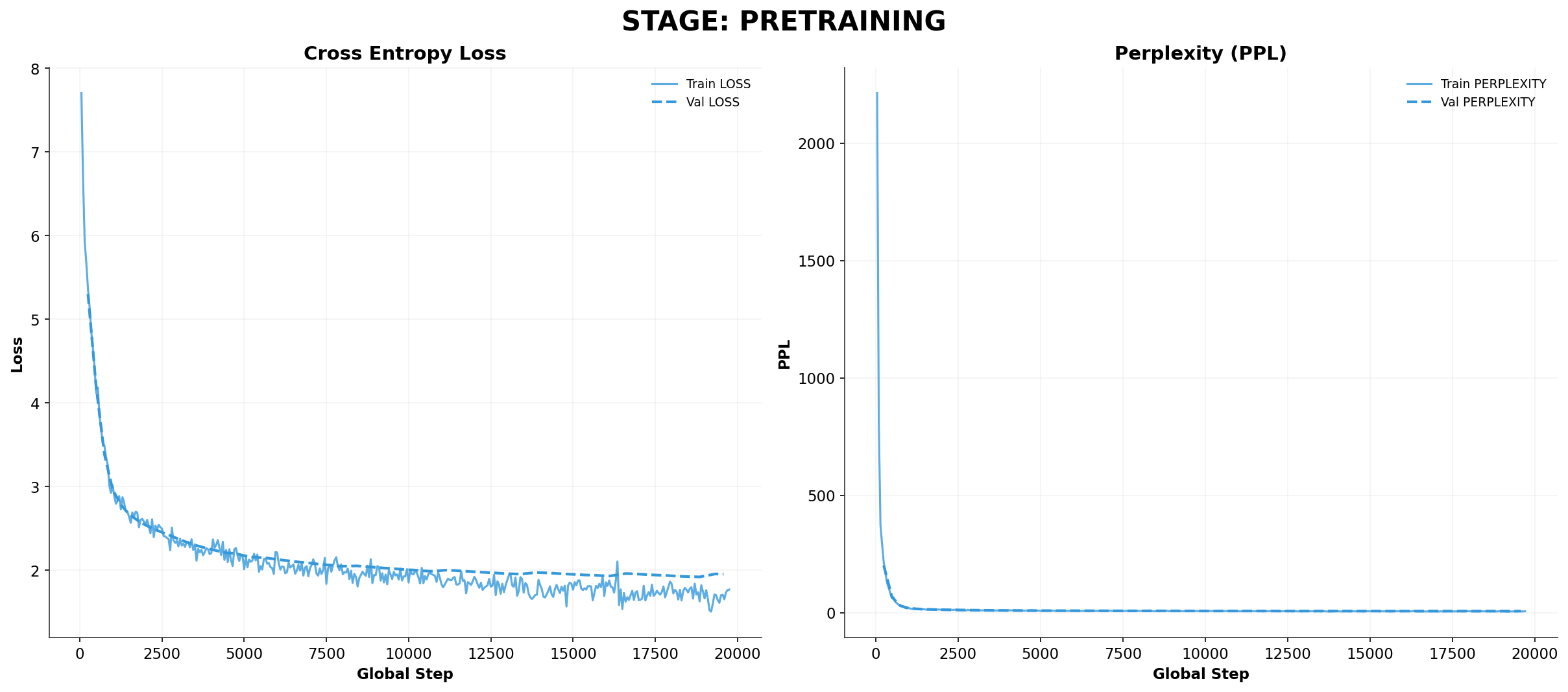 Training history for the best settings
Sample text generation after Pretraining
The figures above illustrate the Autoresearch progress and the training history for the optimal settings. Key architectural optimizations discovered by Autoresearch include:
- Max Sequence Length: Reduced from 1280 to 768 (aligning with the data distribution)
- Hidden Dim: Increased from 1536 to 2048 (a 2.67x ratio)
- Attention Heads: Reduced from 12 to 6 (a head dimension of 128 outperformed 64 in all tests)
- KV Heads: Standardized to 2 (GQA with 3 groups)
Addressing Misaligned Autoresearch Objectives
In the Autoresearch progress plot, you may notice an increase in validation loss after Experiment 30. This occurred because, starting at Experiment 21, the agent learned that reducing model depth lowered validation loss. Since I had not yet specified that the model required reasoning capabilities, it began sacrificing depth to minimize loss. I then intervened to update the objective, guiding the agent back in the right direction.
Be very specific about what you want the model to achieve. Otherwise, the agent will find shortcuts to reach the assigned objective, which may not align with your goals.
Supervised Fine-Tuning (SFT) - Learning to Converse
In this stage, the base model is fine-tuned on a high-quality instructional dataset to learn conversational formats and follow human instructions. We utilized 25,700 samples from the STE SFT dataset. While we limited the Pretraining Autoresearch phase to 20 minutes, we allowed the SFT, Alignment, and Reasoning Autoresearch phases to run until the completion of training. During SFT, Autoresearch focused primarily on optimizing learning rates and WSD scheduler settings. Many initial trials (conducted during the V1 phase of Autoresearch, not shown below) were discarded due to the low quality of generated samples.
| Hyperparameter | Value |
|---|---|
| Dataset | 25,700 samples |
| Batch Size | 16 (Accum=4, Effective=64) |
| Learning Rate | |
| Epochs | 5 |
| Total Steps | ~1,988 Optimizer Steps (Best ckpt at 800 steps) |
| Scheduler | Cosine with 100 Warmup Steps |
| Weight Decay | 0.01 |
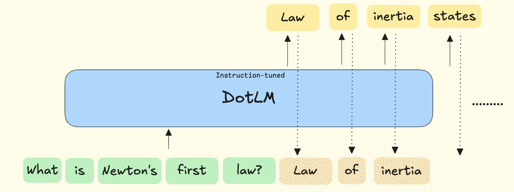 Sample text generation after SFT
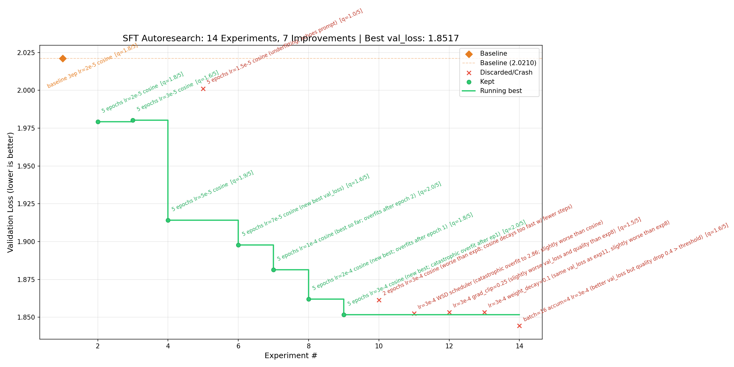 Autoresearch progress during SFT
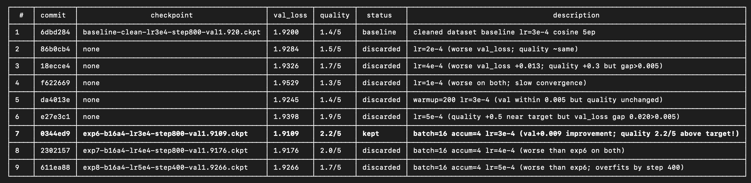 Changes in training settings during SFT
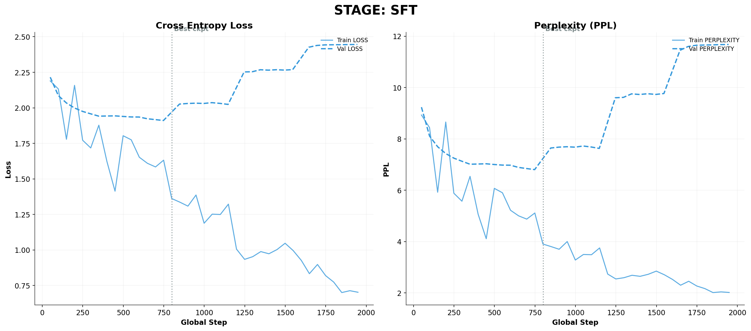 Training history for the best settings
Sample text generation after SFT
Alignment - Adhering to Human Preferences
Alignment via Direct Preference Optimization (DPO) ensures the model's outputs reflect human intent and preferences. Since each training sample contains both a "chosen" and a "rejected" response, the memory requirement per sample is effectively doubled. During this stage, we observed a significant negative correlation between validation loss and the quality of generated samples: across all experiments, the quality of generated samples degraded even as validation loss continued to improve.
Standard hyperparameter tuning typically fails to address such inverse relationships; this is precisely where Autoresearch excels.
| Hyperparameter | Value |
|---|---|
| Dataset | 7,172 samples |
| Batch Size | 8 (Accum=4, Effective=32) |
| Learning Rate | |
| DPO Beta | 0.2 (Strong preference signal) |
| Epochs | 10 |
| Total Steps | ~2,220 Optimizer Steps (Best ckpt at 600 steps) |
| Scheduler | Cosine with 111 Warmup Steps |
| Val Steps | 300 (~3 checks/epoch) |
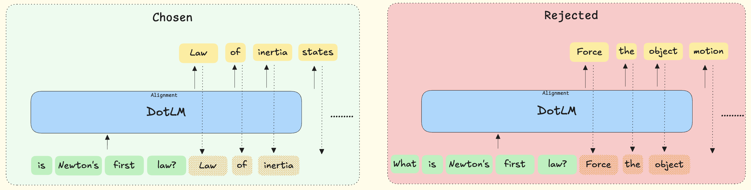 Sample text generation after Alignment
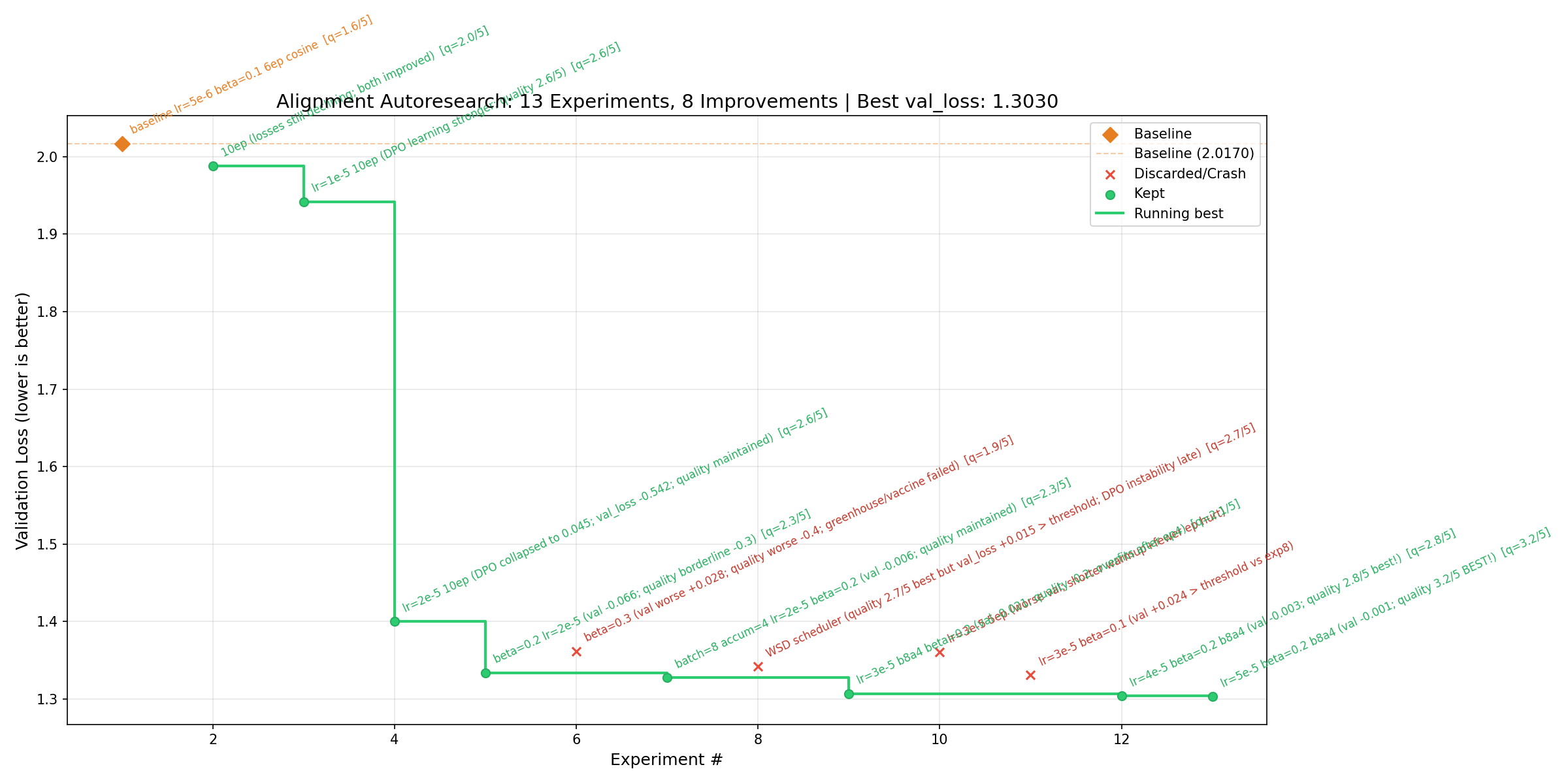 Autoresearch progress during Alignment
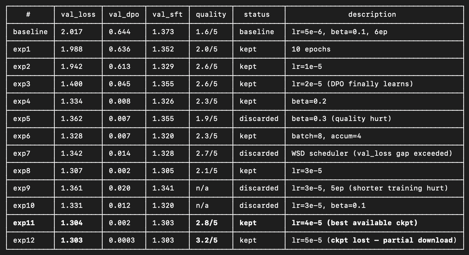 Changes in training settings during Alignment
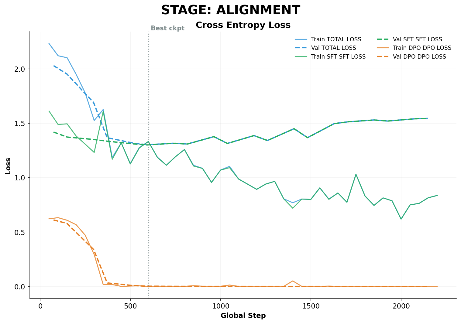 Training history for the best settings
Sample text generation after Alignment
Reasoning - Thinking Before Speaking
The final stage involves training the model to generate Chain-of-Thought (CoT) reasoning enclosed in <think>...</think> tags. This phase utilizes a specialized reasoning dataset with compressed thought traces and outputs to fit within the 768-token context window. During this stage, Autoresearch varied the learning rate and scheduler parameters simultaneously, in contrast to the SFT phase where the learning rate was optimized independently at the start.
| Hyperparameter | Value |
|---|---|
| Dataset | 6,300 samples |
| Batch Size | 16 (Accum=2, Effective=32) |
| Learning Rate | |
| Epochs | 10 |
| Total Steps | ~1,940 Optimizer Steps (Best ckpt at 800 steps) |
| Scheduler | Cosine with 50 Warmup Steps |
| Weight Decay | 0.01 |
| Val Steps | 200 (~2 checks/epoch) |
How Autoresearch Refined the Training Objective
Initially, the objective was set to minimize validation loss while maximizing the quality of generated samples. However, the agent observed that certain training configurations resulted in outputs missing the required </think> closing tag. Consequently, the agent updated its objective to discard settings that failed to reliably close the reasoning block. This was one of the most significant modifications the agent introduced during the reasoning step, as it directly improved the model's structural coherence and reasoning performance.
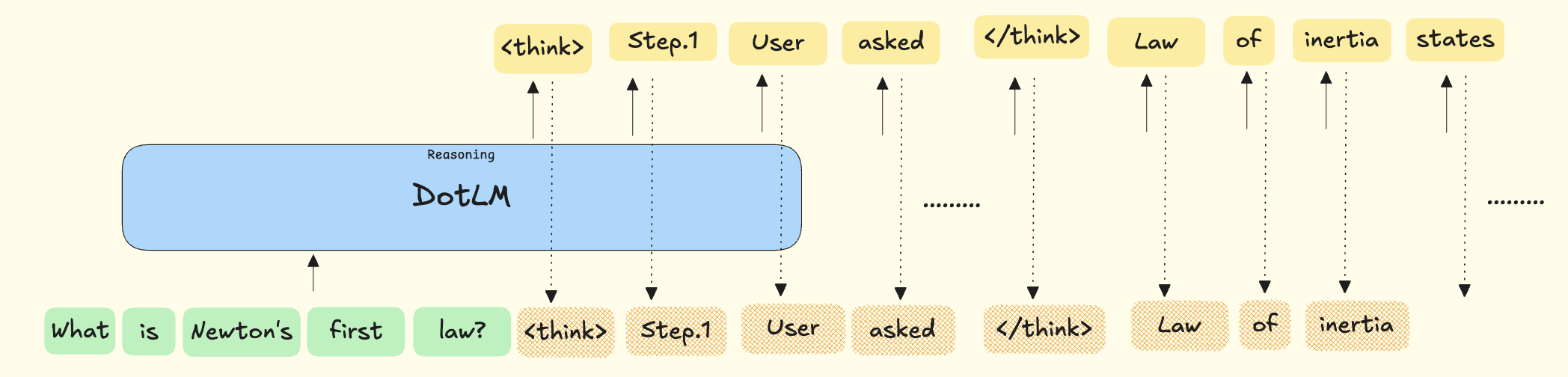 Sample text generation after Reasoning
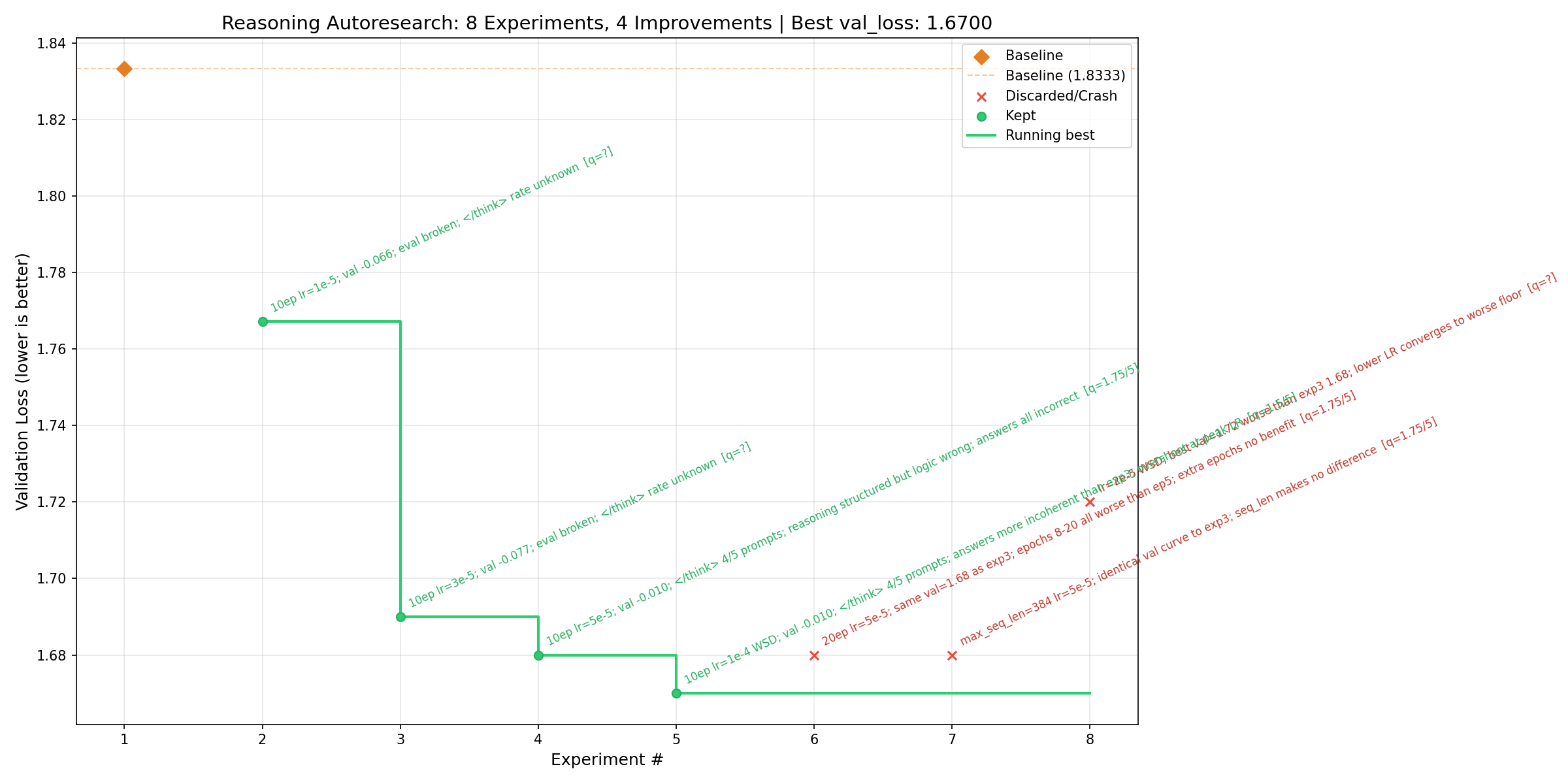 Autoresearch progress during Reasoning
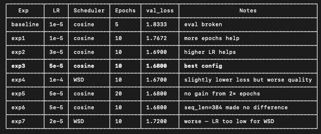 Changes in training settings during Reasoning
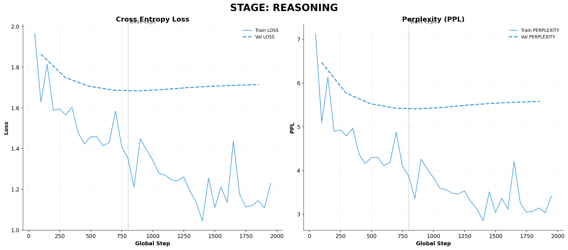 Training history for the best settings
Sample text generation after Reasoning
Inference Optimization
Existing Methods
Quantization
Quantization reduces the precision of the model's weights (e.g., from 16-bit floats like FP16 or BF16 to 8-bit or 4-bit integers like INT8 or INT4). This sharply decreases the memory footprint and increases the memory bandwidth utilization, allowing for faster generation times and the ability to run on consumer hardware with less VRAM, often with negligible degradation in model quality.
Flash Attention
Flash Attention is a hardware-aware exact attention algorithm. It optimizes memory access patterns by tiling the attention computation, which drastically reduces the number of read/write operations to the GPU's High-Bandwidth Memory (HBM). This results in much faster execution and significantly lower memory consumption compared to standard attention implementations, particularly for long context lengths.
KV Cache
The KV Cache stores the computed Key () and Value () representations of previous tokens during autoregressive generation. Since predicting the next token requires attention over all preceding tokens, caching these values instead of recomputing them at every step transforms an generative computation cost into an operation per step.
- Static KV Cache: Pre-allocates a fixed memory buffer for the maximum supported sequence length. This approach eliminates the overhead of dynamic allocation during generation and ensures deterministic memory usage, though it can be wasteful for shorter sequences.
- Dynamic KV Cache: Allocates memory for KV pairs on-the-fly, typically managed through paging mechanisms like PagedAttention. This significantly reduces memory fragmentation and allows for higher batch sizes and throughput by only consuming memory proportional to the actual sequence length.
Speculative Decoding
Speculative Decoding is a latency optimization technique that employs a smaller, faster "draft" model alongside the larger target LLM. The draft model rapidly generates a sequence of potential next tokens. The target model then verifies these tokens efficiently in a single forward pass. Tokens that are accepted are yielded immediately, which allows multiple tokens to be produced per step and significantly accelerates inference without altering the final output probabilities.
Paged Attention
Inspired by virtual memory paging in operating systems, Paged Attention splits the contiguous KV cache into fixed-size blocks ("pages") allocated dynamically in non-contiguous memory spaces. This largely eliminates memory fragmentation and avoids pre-allocating worst-case sequence lengths, which substantially increases the maximum batch size and throughput when serving LLMs concurrently.
CUDA Graphs
CUDA Graphs optimize the CPU overhead of launching GPU kernels. In traditional execution, the CPU must launch each kernel layer by layer, which introduces a latency bottleneck, especially for small models or small batch sizes where GPU execution outpaces the CPU launch time. CUDA Graphs record the entire sequence of GPU operations into a single topological graph and launch it with a single CPU instruction, effectively removing kernel launch latency overhead.
DotLM Inference Analysis
Speculative decoding works best when the draft model is significantly faster (e.g., 10-100x) than the target model. In the case of DotLM, using a draft model is impractical due to the model's already small size. Small models like DotLM are primarily compute-bound rather than memory-bound; the overhead of non-contiguous memory access can degrade performance, whereas simple linear memory access is much faster.
I conducted an extensive analysis of DotLM inference performance on an NVIDIA L40S GPU by combining several optimization techniques: Quantization, Flash Attention, KV Caching, and CUDA Graphs. I evaluated both FP32 and BF16 precision models, as 8-bit or 4-bit quantization might not be necessary for a model of this scale. The figure below compares the throughput and memory usage across various DotLM configurations.
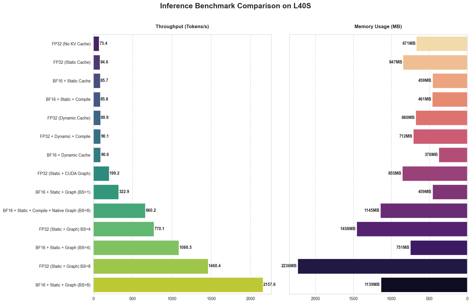 DotLM Inference benchmarking
The combination of the BF16 precision model with a Static KV Cache and CUDA Graphs (using a batch size of 8) yielded the best throughput at 1460 tokens/sec with a memory footprint of 1139MB. CUDA Graphs notably improved throughput with only a marginal increase in memory usage.
Evaluation
DotLM was evaluated against multiple benchmarks to assess its performance across diverse tasks. Results are compared against the GPT-2 baseline (with Qwen 0.5B included for reference) to contextualize the improvements realized by DotLM.
1. Commonsense and Linguistic Reasoning
- HellaSwag: This task requires the model to predict the most plausible ending to a sentence. Scoring 32% is a significant improvement over the GPT-2 baseline (~29%), demonstrating that the model understands physical and social contexts.
- Winogrande: Focused on pronoun resolution. While DotLM slightly outperforms GPT-2 at 52%, it remains just 2% above random chance, placing it in the realm of borderline random guessing.
2. Academic Scientific Knowledge
- SciQ: This is where DotLM-165M truly shines. Outperforming GPT-2 by 8%, the model demonstrates a strong ability to retrieve scientific facts and textbook knowledge.
- ARC-Easy: In grade-school science questions, DotLM again leads the GPT-2 baseline. This suggests that smaller models can excel as "compact encyclopedias" when trained on high-quality, high-density data.
3. The Reasoning Frontier
- GPQA: GPQA is designed to be "Google-proof," often requiring expert-level knowledge. A score of 22% (slightly below random) is entirely expected at this scale. Mastery of expert reasoning remains the primary differentiator between sub-billion parameter models and large-scale LLMs.
| Benchmark | GPT-2 (124M) | DotLM (165M) | Qwen (500M) |
|---|---|---|---|
| HellaSwag | 29.0% | 32.0% | 48.0% |
| ARC-Easy | 40.0% | 42.0% | 60.0% |
| Winogrande | 50.2% | 52.0% | 56.2% |
| SciQ | 50.0% | 58.0% | 85.0% |
| GPQA | 24.0% | 22.0% | 26.5% |
DotChat - The ChatUI for DotLM
DotChat is a chat interface built to interact with DotLM-165M. It consists of a Next.js frontend deployed on Vercel and a Python backend deployed on Modal as a serverless GPU endpoint. The backend exposes a single streaming endpoint via FastAPI and Server-Sent Events (SSE), keeping the architecture minimal and cost-efficient.
Inference Stack
The backend inference pipeline is composed of three main modules: Tokenizer, Inference Engine, and Chat Manager. On container startup, the engine loads the model weights from a persistent Modal Volume and initializes the chat manager. The model stays warm in memory for 180 seconds between requests, eliminating repeated cold-start overhead for active user sessions.
Streaming Token Generation
The inference engine drives generation token-by-token using a manual KV cache loop. This avoids the overhead of a standard model.generate() call and enables true streaming:
- Prefill: The full conversational prompt is passed in one forward pass, populating the KV cache for all layers.
- Decode loop: Each subsequent step feeds only the single most-recent token, with the KV cache providing the full attention history.
- Incremental Decoding: The output tokens are dynamically decoded and mapped back to strings, allowing the server to stream chunks of text immediately via a Server-Sent Events connection.
Adding Conversational Capabilities
Maintaining a coherent conversation is one of the most significant challenges for Small Language Models (SLMs). Models with fewer parameters are highly sensitive to noise in the prompt and easily get "confused" when forced to process long, irrelevant historical context. If you simply append the entire chat history to a 165M model, it often begins to hallucinate or lose focus on the current query.
To solve this, DotChat uses a Dynamic Context Injection approach. Instead of blindly passing history, the system performs a real-time "topic shift" analysis to decide if the previous turn is actually relevant to the current user query.
The Topic Classification
When a user sends a query in conversational mode, the ChatManager executes two very fast, partial inference passes (generating only ~15 tokens) to extract Topic Vectors:
Query Only: A vector representing the semantic intent of the query in isolation.Query + Previous Response: A vector representing the intent when the query is prefixed with the previous assistant's response.
By calculating the Cosine Similarity between these two vectors, we can determine if the conversation is still on the same topic.
- Similarity ≥ 0.5: The query is semantically linked to the previous answer. A truncated version of the previous response is injected as a context prefix.
- Similarity < 0.5: A topic shift is detected. The query is treated as a fresh start, and no context is injected.
This approach ensures that DotLM-165M only receives the context it needs to stay coherent, effectively bypassing its inherent small-scale context limitations. Though it's not as good as LLMs, it seems to work well for most of the queries that I have tested.
Conversational Pipeline Flowchart
 DotChat Conversational Pipeline Flowchart
ChatUI Details
The frontend is a Next.js app that consumes the Server-Sent Events (SSE) stream and updates the user interface in real time. It parses incoming text chunks and dynamically separates the <think>…</think> reasoning block from the final answer, giving users complete visibility into the model's thought process.
How much did it cost?
- Data Creation: Data is created using APIs from OpenAI, Openrouter and Deepinfra. Total cost is approximately $170.
- Training: All the Autoresearch runs are performed on a single NVIDIA H100 GPU from JarvisLabsAI. The total cost of training DotLM-165M is approximately $150.
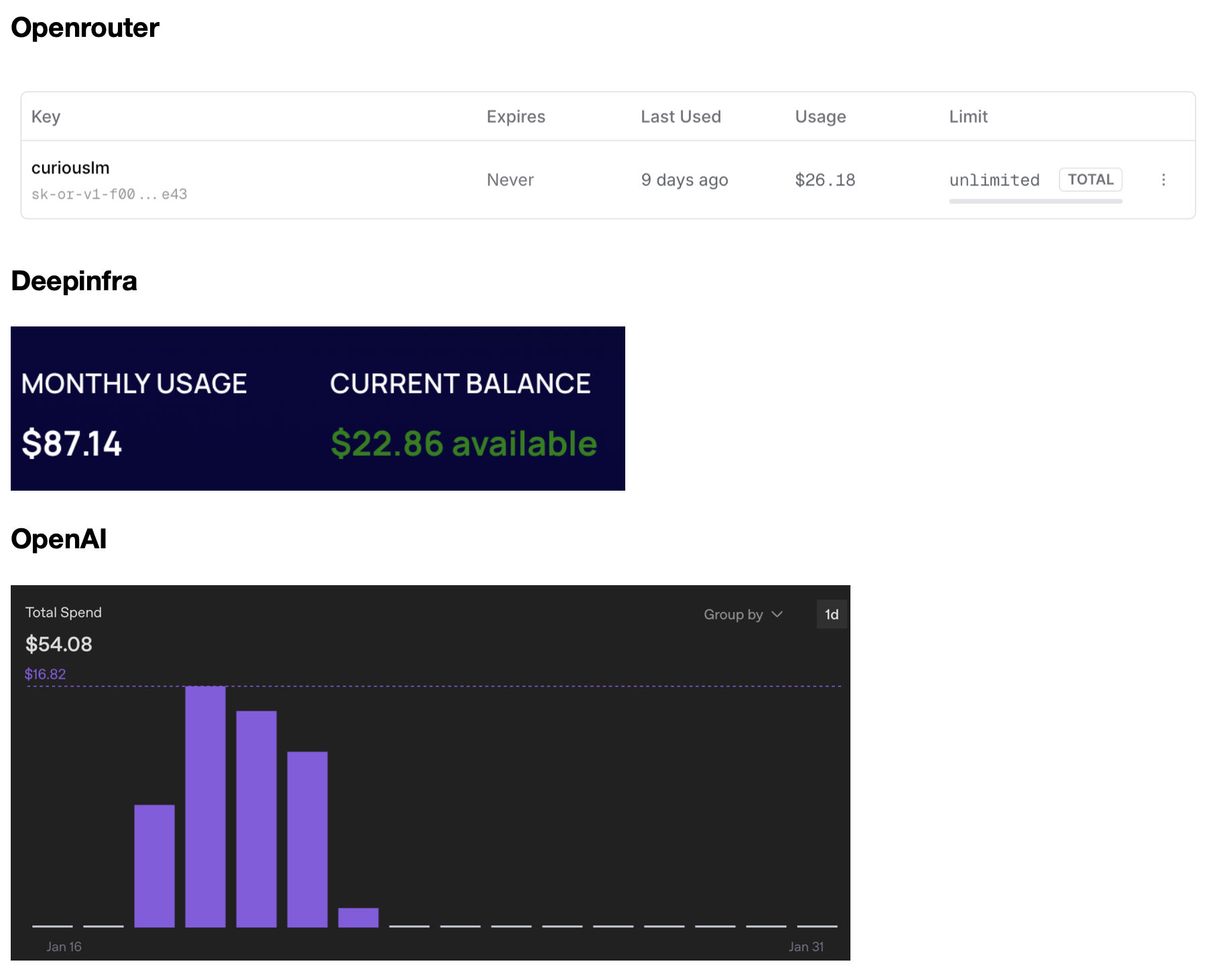 Costs of Data Creation
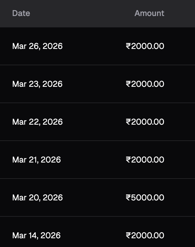 Costs of Training of all Autoresearch runs
Costs of Data Creation
References
- UTF Encoding from HubSpot
- BPE Tokenizer from scratch from Sebastian Raschka
- Grouped Query Attention
- RoPE from LabML
- Weights & Biases - Experiment tracking and visualization
- Autoresearch - Andrej Karpathy's autoresearch project
- Smol training playbook from HuggingFace
- LLMs from scratch by Sebastian Raschka
- KV Cache from HuggingFace
- Speculative Decoding
- Paged Attention from vLLM
- CUDA Graphs
- Qwen 2 Technical Report
- GPT-2 Paper
Tools
- JarvisLabsAI - Cloud GPU provider
- Modal - Serverless GPU platform for DotChat
- Vercel - Frontend deployment for DotChat
- Excalidraw - Diagramming tool
- HuggingFace - Model and dataset sharing
- Weights & Biases - Experiment tracking and visualization
- Cloudflare - Domain for DotChat
Citation
Shanmukha Sainath. "DotLM-165M: How I trained a 165M parameter language model from scratch". TensorWrites (Apr 2026). https://www.tensorwrites.com/posts/dotlm
@article{dotlm2026,
  title   = "DotLM-165M: How I trained a 165M parameter language model from scratch",
  author  = "Shanmukha Sainath",
  journal = "TensorWrites",
  year    = "2026",
  month   = "Apr",
  url     = "https://www.tensorwrites.com/posts/dotlm"
}